Homoclinic Orbit and Heteroclinic Orbit
Definition1
Let the space $X$ and the function $f : X \to X$ be given. Consider the following vector field presented in the form of a differential equation. $$ \dot{x} = f(x) $$ A flow of this system can be represented as $\phi (t, x)$.
Homoclinic Orbit
For a certain fixed point $x_{0}$, a curve satisfying the following $\phi$ is called a homoclinic orbit. $$ \lim_{t \to \pm \infty} \phi ( t , x ) = x_{0} $$
Heteroclinic Orbit
For two different fixed points $x_{1} \ne x_{2}$, a curve satisfying the following $\phi$ is called a heteroclinic orbit. $$ \begin{align*} \lim_{t \to - \infty} \phi ( t , x ) =& x_{1} \\ \lim_{t \to + \infty} \phi ( t , x ) =& x_{2} \end{align*} $$
Explanation
As the names suggest, a homoclinic orbit converges to the same fixed point both forward and backward in time, hence the prefix homo. On the other hand, a heteroclinic orbit converges to different fixed points, hence the prefix hetero.

Although not directly mentioned in the definition, a homoclinic orbit must have both an entry and an exit path at $x_{0}$, making it a saddle. Meanwhile, a heteroclinic orbit must be an unstable manifold from the exit side at $x_{1}$ and a stable manifold from the entry side at $x_{2}$.
Visualization
Although it is easy to visualize a heteroclinic orbit flowing from one point to another, it is not intuitive to visualize a homoclinic orbit, which includes a closed curve and saddles.
$$ \begin{align*} \dot{x} =& \sigma_{1} x + y \\ \dot{y} =& \left( \sigma_{2} - \sigma_{1} \right) y + \alpha x^{2} - \zeta xy \end{align*} $$
For example, in the given system where $\sigma_{1} = \alpha = \zeta = 1$ and $\sigma_{2} \approx -0.755$, let’s visualize only the homoclinic orbit that appears in the system23.

If you plot the flow from initial points inside the orbit in a video, it looks like this:
Code
The following Julia code generates the data used in this post.
using Plots, LinearAlgebra
μ = -1.755
h = 0.1

f(v) = [v[1] + v[2], μ*v[2] + v[1]^2 - v[1]*v[2]]
pos = Base.product(-1.5:h:.5, -.5:h:2)
dir = f.(pos) ./ 10norm.(f.(pos))

v_ = [[-0.5,0.5]]
for _ in 1:500000
    push!(v_, v_[end] + 0.0001f(v_[end]))
end
truncated_v_ = v_[340000:460000]

p1 = quiver(first.(pos), last.(pos), quiver = (first.(dir), last.(dir)),
xlabel = "x", ylabel = "y", color = :gray, size = [600, 600])
p1 = plot(p1, first.(truncated_v_[1:60000]), last.(truncated_v_[1:60000]), color = :black, lw = 2, label = "orbit", arrow = true)
p1 = plot(p1, first.(truncated_v_[60001:80000]), last.(truncated_v_[60001:80000]), color = :black, lw = 2, label = :none, arrow = true)
p1 = plot(p1, first.(truncated_v_[80001:90000]), last.(truncated_v_[80001:90000]), color = :black, lw = 2, label = :none, arrow = true)
p1 = plot(p1, first.(truncated_v_[90001:120000]), last.(truncated_v_[90001:120000]), color = :black, lw = 2, label = :none, arrow = true)
p1 = scatter(p1, [0], [0], color = :black, label = "saddle node", shape = :rect)
png(p1, "saddle_orbit.png")
anim = @animate for tk in 1:1000:460001
    plot(p1, first.(v_[1:100:tk]), last.(v_[1:100:tk]), lw = 1, color = :blue, label = :none, arrow = true)
end
mp4(anim, "saddle_orbit.mp4", fps = 30)
Related Topics
Kuznetsov. (1998). Elements of Applied Bifurcation Theory: p59. ↩︎
Wu. (2000). Homoclinic Bifurcation in an SIQR Model for Childhood Diseases: https://doi.org/10.1006/jdeq.2000.3882 ↩︎
