매키-글래스 방정식
모델
다음과 같이 혈액세포의 생성과 소멸을 묘사하기 위해 제안된 지연미분방정식을 매키-글래스 방정식Mackey–Glass equation이라고 한다1.
$$ \dot{x}(t) = \beta_{0}\frac{ \theta^{n} x(t-\tau)}{ \theta^{n} + x(t-\tau)^n} - \gamma x(t) $$
- $x(t)$: $t$ 시점에서 혈액세포의 양
- $\beta_{0}$: 세포의 생성에 관련된 파라미터
- $\gamma$: 세포의 소멸률
- $\tau$: 생성 과정의 시간 지연
- $n$: 데이터에 피팅하기 위한 파라미터
- $\theta = 1$: 데이터에 피팅하기 위한 파라미터
설명
원논문을 보면 다음과 같이 첫째항의 분자에 $x(t-\tau)$ 가 빠진 것도 같이 고려한다. $$ \dot{x}(t) = \beta_{0}\frac{ \theta^{n} }{ \theta^{n} + x(t-\tau)^n} - \gamma x(t) $$
혼돈
세포는 과거의 $x(t-\tau)$ 와 함께 홀링타입 반응과 유사한 곡선을 따라 생성되고, 현재 양에 비례해서 소멸하는 것으로 가정한다.
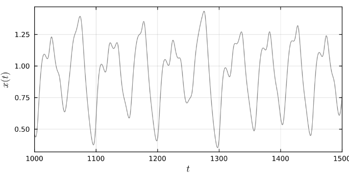
해서 $x$ 는 1차원 공간을 다루고 있음에도 위와 같이 캐어릭한 양상을 보인다. 기본적으로는 위아래로 오실레이션oscillation이 반복된다.
지연좌표
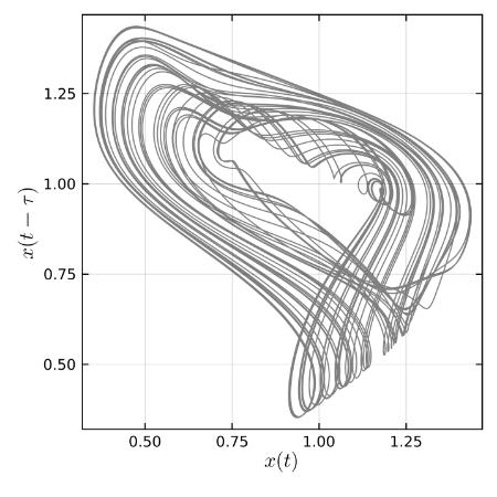
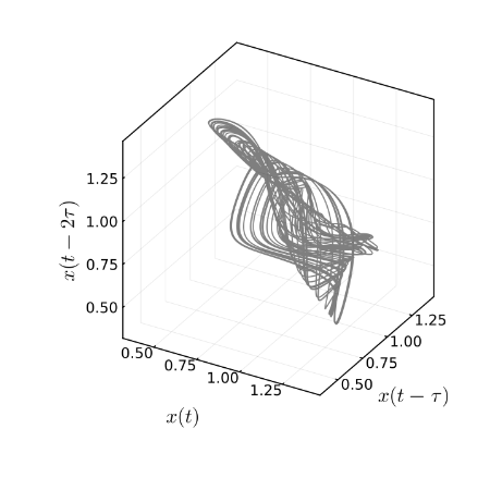
실제로도 같은 해에서 서로 다른 시점의 값을 가져와 $y = x(t-\tau)$ 라 두면 마치 이상한 어트랙터처럼 보이는 궤적을 얻을 수 있다. $z = x(t-2\tau)$ 까지 가져오면 3차원 공간에서의 궤적도 볼 수 있다.
바이퍼케이션
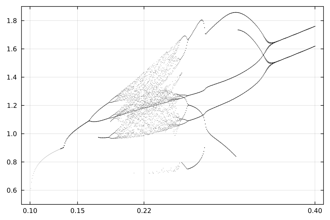
$\beta_{0} \in [0.15, 0.40]$ 에서 $x$ 의 로컬맥시마를 모아서 그린 바이퍼케이션 다이어그램이다.
코드
다음은 줄리아로 매키-글래스 방정식을 풀고 시계열과 지연좌표의 궤적을 그리는 코드다. $\tau=17$, $\gamma=0.1$, $n=10$, $\beta_{0}=0.22$ 로 둔다.
지연미분방정식은 DDEProblem으로 정의하며 초기 이력 phi를 함께 전달한다. 시스템 안의 hist(p, t - τ)는 과거의 상태를 조회하는 함수다.
prob = DDEProblem(sys, [Float64(c)], phi, (0.0, Float64(last(saveat))), [β0]; constant_lags = [τ])
sol = solve(prob, MethodOfSteps(RK4()); dt, adaptive = false, maxiters = Inf)
아래 전체 코드에서 ic = [a, b, c]는 초기 이력의 세 점 $\phi(-\tau)=a$, $\phi(-\tau/2)=b$, $\phi(0)=c$ 를 지정한다. 세 점은 직선으로 연결하며, 모두 같게 두면 일정한 초기 이력이 된다.
saveat = 1000:1e-2:3000은 $t=0$ 부터 계산한 해에서 $t=1000$ 이후의 데이터만 가져오겠다는 의미다. 반환되는 열은 순서대로 시간, 세 좌표, 각 좌표의 미분계수다.
전체 코드
using DifferentialEquations, DataFrames, Plots, LaTeXStrings, DelayDiffEq
using OrdinaryDiffEqLowOrderRK: RK4

function factory_macglas(β0::Number; ic = [1.2, 1.2, 1.2], saveat = 0:1e-2:100)
    τ, γ, n = (17, 0.1, 10)
    a, b, c = ic isa Number ? (ic, ic, ic) : ic
    dt = step(saveat)

    function sys(du, u, hist, p, t)
        xτ = hist(p, t - τ)[1]
        du[1] = p[1]*xτ/(1 + xτ^n) - γ*u[1]
        return du
    end
    phi(p, t) = t ≤ -τ/2 ? [a + (b - a)*(t + τ)/(τ/2)] : [b + (c - b)*(t + τ/2)/(τ/2)]
    dphi(t) = t ≤ -τ/2 ? (b - a)/(τ/2) : (c - b)/(τ/2)

    prob = DDEProblem(sys, [Float64(c)], phi, (0.0, Float64(last(saveat))), [β0]; constant_lags = [τ])
    sol = solve(prob, MethodOfSteps(RK4()); dt, adaptive = false, maxiters = Inf)

    xat(t) = t < 0 ? phi(nothing, t)[1] : sol(t; idxs = 1)
    dxat(t) = t < 0 ? dphi(t) : β0*xat(t - τ)/(1 + xat(t - τ)^n) - γ*xat(t)

    t = collect(saveat)[1:end-1]
    x  = xat.(t)
    y  = xat.(t .- τ)
    z  = [s ≥ τ ? xat(s - 2τ) : NaN for s in t]
    dx = dxat.(t)
    dy = dxat.(t .- τ)
    dz = [s ≥ τ ? dxat(s - 2τ) : NaN for s in t]
    return [t x y z dx dy dz]
end
factory_macglas(T::Type, args...; kargs...) =
DataFrame(factory_macglas(args...; kargs...), ["t", "x", "y", "z", "dx", "dy", "dz"])

sol = factory_macglas(DataFrame, .22, saveat = 1000:1e-2:3000)
plot(sol.t, sol.x, alpha = .5, color = :black, legend = false, xlabel = L"t", ylabel = L"x(t)", size = [600, 300], xlim = [1000, 1500])
plot(sol.x, sol.y, alpha = .5, color = :black, legend = false, xlabel = L"x(t)", ylabel = L"x(t-\tau)", size = [400, 400])
plot(sol.x, sol.y, sol.z, alpha = .5, color = :black, legend = false, xlabel = L"x(t)", ylabel = L"x(t-\tau)", zlabel = L"x(t-2\tau)", size = [400, 400])
참고로 초기 이력을 $[-\tau,0]$ 에서만 지정했으므로 $t<\tau$ 에서는 $x(t-2\tau)$ 를 구할 수 없다. 이 구간의 z, dz는 NaN으로 둔다.
Mackey, Michael C., and Leon Glass. “Oscillation and chaos in physiological control systems.” Science 197.4300 (1977): 287–289. https://doi.org/10.1126/science.267326 https://www.mcgill.ca/mathematical-physiology-lab/files/mathematical-physiology-lab/1977jul_mcm_glass_oscillation_chaos_physiological_ctrl_syst.pdf ↩︎