
How to Read Logistic Regression Results in R
Practice
Let’s load the built-in data turnout.
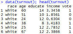
turnout is data on the 1992 US general election, from which one can examine vote (whether one voted) according to race, age, educate (education level), and income. Since this data is concerned with the dependent variable of whether one voted or not, logistic regression can be used.
Unlike ordinary regression analysis, logistic regression builds a model through the glm() function. If you add family=binomial() as an option, it performs logistic regression automatically. The reason ‘binomial’ suddenly appears is that the dependent variable is a binomial variable taking 0 or 1.
Interpreting the Results
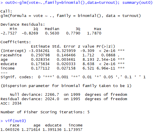
Looking at the results, they are similar to ordinary multiple regression analysis yet differ in many respects. The way to read the regression coefficients for each variable is the same, but the F-test is gone and something called deviance has appeared.
Deviance can safely be regarded as a measure of how poorly the logistic regression model explains the data. The null deviance is the deviance when there are no variables at all and only the constant term, which can be seen as the worst-case situation of having no data whatsoever. The residual deviance obtained this way is the smaller the better, and since it follows a chi-squared distribution, one can check whether the model fits through a chi-squared goodness-of-fit test.
Although the name of the glm() function means ‘generalized regression analysis’, since it is fundamentally regression analysis, multicollinearity cannot be ignored. Fortunately, the VIF can be easily obtained by using the vif() function. In the example, there appears to be no multicollinearity problem.
Model Diagnostics
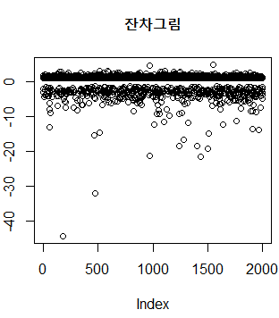
On the other hand, the residual plot is quite shocking, but fortunately, in logistic regression the residual plot carries no meaning at all. Therefore, there is no need to bother checking it, and even if it looks strange when you do check, there is no need to worry. The goodness-of-fit test mentioned earlier is sufficient.
Now let’s actually check whether the model fits through several methods.

The way to perform a chi-squared goodness-of-fit test is very simple. If you want to test at significance level $\alpha$, you compute the critical value by plugging $(1 - \alpha)$ and the degrees of freedom of the residual deviance into the qchisq() function. If the residual deviance is smaller than the critical value as above, the model is considered to fit.
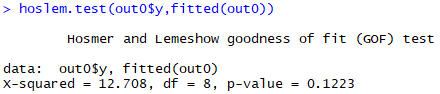
The Hosmer-Lemeshow goodness-of-fit test is a representative goodness-of-fit test used in logistic regression, which likewise tests whether the model fits through a chi-squared statistic. It can be tested by plugging the model’s actual dependent variable and fitted values into the hoslem.test() function of the ResourceSelection package. Since the null hypothesis is ’the model fits’, if the p-value is high and the null hypothesis cannot be rejected as above, the model is considered to fit. However, according to Frank Harrell, it has various weaknesses and is now no longer recommended1.
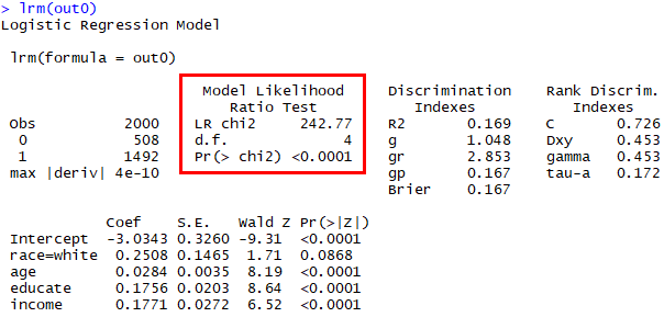
Using the lrm() function of the rms package performs a likelihood ratio test of the model. Unlike the two methods above, which are goodness-of-fit tests with the null hypothesis ’the model fits’, in the likelihood ratio test the model is considered to fit when the null hypothesis is rejected. If you are using the rms package anyway, there is no need to build a logistic regression model with the glm() function and feed in its output—you may just put the model directly into the lrm() function. In the example, entering lrm(vote~.,data=turnout) performs the entire process at once.
Prediction
Finally, let’s compute probabilities directly using the logistic regression model. The probabilities are computed simply by adding the type='response' option to the predict() function.
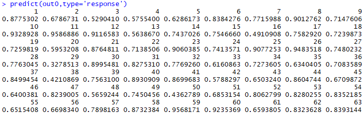
Of course, since we already have the data and know the true values, such prediction is not very meaningful. Therefore, a process of giving new data through the newdata option and checking whether it still predicts well is necessary.
Code
Below is the example code.
install.packages("Zelig")
install.packages("car")
install.packages("ResourceSelection")
install.packages('rms')

library(Zelig)
data(turnout); head(turnout)
out0<-glm(vote~.,family=binomial(),data=turnout); summary(out0)

library(car)
vif(out0)

win.graph(4,4); plot(out0$residuals,main="잔차그림")

qchisq(0.95,df=1995)

library(ResourceSelection)
hoslem.test(out0$y,fitted(out0))

library(rms)
lrm(out0)
lrm(vote~.,data=turnout)

predict(out0,type='response\')