Fourth-Order Runge-Kutta Method 📂Numerical Analysis

Fourth-Order Runge-Kutta Method

Method¹

For a continuous function $f$ defined on $D \subset \mathbb{R}^2$, suppose the initial value problem $\begin{cases} y ' = f(x,y) \\ y( x_{0} ) = Y_{0} \end{cases}$ is given. Suppose the interval $(a,b)$ is partitioned into node points such that $a \le x_{0} < x_{1} < \cdots < x_{n} < \cdots x_{N} \le b$. In particular, if $x_{j} = x_{0} + j h$ for sufficiently small $h > 0$, then for the initial value $y_{0} = Y_{0}$ $$ y_{n+1} = y_{n} + h \sum_{j=1}^{p} \gamma_{j} V_{j} $$

Explanation

The Runge-Kutta method, like the Adams method, comes in various forms, and $\gamma_{j}$ and $V_{j}$ are determined through complicated algebraic manipulations. Among them, the most popular one is the fourth-order Runge-Kutta method, commonly abbreviated as RK4.

Fourth-order Runge-Kutta method: $$ \begin{align*} y_{n+1} =& y_{n} + {{h} \over {6}} \left[ V_{1} + 2 V_{2} + 2 V_{3} + V_{4} \right] \\ V_{1} =& f(x_{n} , y_{n}) \\ V_{2} =& f \left( x_{n} + {{h} \over {2}} , y_{n} + {{h} \over {2}} V_{1} \right) \\ V_{3} =& f \left( x_{n} + {{h} \over {2}} , y_{n} + {{h} \over {2}} V_{2} \right) \\ V_{4} =& f \left( x_{n} + h , y_{n} + h V_{3} \right) \end{align*} $$

Looking at the formulas, one can see that in order to advance by a single step $h$, even the data at the point $\displaystyle {{h} \over {2}}$ is used. For a more generalized explanation, refer to See Also.

Intuitive Derivation

Let us unpack the terms above one by one and think about them through the simplest Euler method $y_{n+1} = y_{n} + h f ( x_{n} , y_{n} ) $. (For convenience, let $\displaystyle x_{n+ {{1} \over {2}} } : = x_{n} + {{h} \over {2}}$, $y_{n+ {{1} \over {2}} } \approx Y(x_{n + {{h} \over {2}} } )$.) $$ V_{1} = f(x_{n} , y_{n} ) $$ becomes the derivative $y_{n} ' $ at the point $x_{n}$. $$ \begin{align*} V_{2} =& f \left( x_{n} + {{h} \over {2}} , y_{n} + {{h} \over {2}} f \left( x_{n} , y_{n} \right) \right) \\ =& f \left( x_{n + {{1} \over {2}} } , y_{n + {{1} \over {2}} } \right) \end{align*} $$ becomes the derivative $\displaystyle y_{n + {{1} \over {2}} } ' $ at the point $x_{n+{{1} \over {2}} }$. $$ V_{3} = f \left( x_{n} + {{h} \over {2}} , y_{n} + {{h} \over {2}} f \left( x_{n + {{1} \over {2}} } , y_{n + {{1} \over {2}} } \right) \right) $$ also, by the backward Euler method $y_{n+1} = y_{n} + h f ( x_{n+1} , y_{n+1} )$, becomes $\displaystyle V_{3} = f \left( x_{n + {{1} \over {2}} } , y_{n + {{1} \over {2}} } \right) $, the derivative $\displaystyle y_{n + {{1} \over {2}} } ' $ at the point $x_{n+{{1} \over {2}} }$. $$ \begin{align*} V_{4} =& f \left( x_{n} + h , y_{n} + h V_{3} \right) \\ =& f \left( x_{n} + {{h} \over {2}} + {{h} \over {2}} , y_{n} + {{h} \over {2}} V_{3} + {{h} \over {2}} V_{3} \right) \\ =& f \left( x_{n + {{h} \over {2}}} + {{h} \over {2}} , y_{n + {{h} \over {2}}} + {{h} \over {2}} V_{3} \right) \end{align*} $$ likewise, by the backward Euler method, becomes the derivative $\displaystyle y_{n + 1} ' $ at the point $x_{n+ 1 }$. $$ {{h} \over {6}} \left[ V_{1} + 2 V_{2} + 2 V_{3} + V_{4} \right] $$ can be seen as a weighted average that uses even the data at the point $x_{n+{{1} \over {2}} }$ to advance by a single step $h$, giving particular weight to the point $x_{n+{{1} \over {2}} }$.

More computations could be added here, but from RK4 onward, the order of convergence does not increase as much as the amount of computation. Even without pushing it further, RK4 alone tends to be sufficient unless the problem is stiff, and coding it is also relatively easy, which is why it is widely used.

Implementation

R

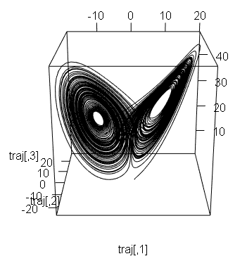
The following is code that implements RK4 in R and draws the Lorenz attractor in 3D.

library(rgl)
 
RK4<-function(ODE,v,h=10^(-2)){
  V1 = ODE(v)
  V2 = ODE(v + (h/2)*V1)
  V3 = ODE(v + (h/2)*V2)
  V4 = ODE(v + h*V3)
  v = v + (h/6)*(V1 + 2*V2 + 2*V3 + V4)
  return(v)
}
 
lorenz<-function(v,rho=28,sigma=10,beta=8/3){
  dvdt = v
  dvdt[1] = sigma*(v[2]-v[1])
  dvdt[2] = v[1]*(rho-v[3])-v[2]
  dvdt[3] = v[1]*v[2] - beta*v[3]
  return(dvdt)
}
 
traj<-numeric(0)
v=c(1,1,1)
for(i in 1:10000){
  traj<-rbind(traj,v)
  v=RK4(lorenz,v)
}
 
plot3d(traj,type='l')
plot(traj[,1],traj[,3],type='l')

Running the code yields the following 3D plot.

$20190226\_173942.png$

Julia

The following is an implementation of the same content in Julia.

using Plots
function RK4(ODE::Function,v::Array{Float64,1},h=10^(-2))
    V1 = ODE(v)
    V2 = ODE(v .+ (h/2)*V1)
    V3 = ODE(v .+ (h/2)*V2)
    V4 = ODE(v .+ h*V3)
    return @. v + (h/6)*(V1 + 2*V2 + 2*V3 + V4)
end
function lorenz(v::Array{Float64,1}; ρ=28.,σ=10.,β=8/3)
  dvdt = deepcopy(v)
  dvdt[1] = σ*(v[2]-v[1])
  dvdt[2] = v[1]*(ρ-v[3])-v[2]
  dvdt[3] = v[1]*v[2] - β*v[3]
  return dvdt
end
function  lorenz_attracter(v::Array{Float64,1}, endtime = 10000)
  x,y,z = [v[1]], [v[2]], [v[3]]
  for t in 1:endtime
    newx,newy,newz = RK4(lorenz,[x[end], y[end], z[end]])
    push!(x, newx)
    push!(y, newy)
    push!(z, newz)
  end
  return x,y,z
end
result = lorenz_attracter([1.,1.,1.])
plot(result)