📂Mathematical Statistics

Credible Interval

Definition ¹

When a subset $C \subset \Theta$ of the parameter space $\Theta$ satisfies $P ( \theta \in C | y ) \ge 1 - \alpha$ with respect to the significance level $\alpha$, $C$ is called a $100(1 - \alpha) %$ credible Interval for $\theta$ given the data $y$.

Explanation

In the Bayesian framework, interval estimation means finding an interval with a high probability of containing the parameter $\theta$. The ‘credible interval’ found in this way is, for a frequentist, the concept corresponding to the confidence interval.

Understanding the Formula

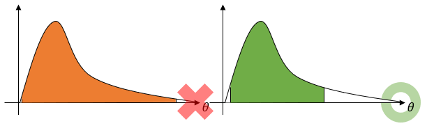
The formula is written in a somewhat difficult way, so let us unpack it. Expressed in integral form, $$ P ( \theta \in C | y ) = \int_{ \theta \in C} p ( \theta | y) d \theta $$ To aid understanding, if we simply set the significance level to $\alpha = 0.05$, then $C$ is called a credible interval when $$ \int_{ \theta \in C} p ( \theta | y) d \theta \ge 0.95 $$ holds. Rewriting it in a slightly more familiar expression as $C = [a,b] $, we get $$ \int_{a}^{b} p ( \theta | y) d \theta \ge 0.95 $$ In the two figures below, if the area of the shaded region is greater than or equal to $0.95$, then this integration interval $C$, whatever it may be, becomes a credible interval.

However, since a credible interval is more accurate the shorter its length is, among the credible intervals that satisfy the condition the smallest one is best. Therefore, if we had to choose one of the two, it would be the one on the right, and in actual estimation a more accurate method is used.

A Conservative Definition

The reason the credible interval is defined as $P ( \theta \in C | y ) \ge 1 - \alpha$ rather than exactly $P ( \theta \in C | y ) = 1 - \alpha$ is simply to be safe. Since there are cases where the calculation cannot be matched exactly, rather than narrowing the interval and getting it wrong, we set it slightly wider.

Looking at this, one might increasingly wonder how it differs from the frequentists’ confidence interval and whether it really needs to be defined anew. But this seemingly subtle difference is precisely one of the core elements that make the Bayesian approach appealing.