📂Numerical Analysis

Trapezoidal Method

Definition¹

Suppose the initial value problem $\begin{cases} y ' = f(x,y) \\ y( x_{0} ) = Y_{0} \end{cases}$ is given for a continuous function $f$ defined on $D \subset \mathbb{R}^2$. Say the interval $(a,b)$ is divided into node points such as $a \le x_{0} < x_{1} < \cdots < x_{n} < \cdots x_{N} \le b$. In particular, if we let $x_{j} = x_{0} + j h$ for sufficiently small $h > 0$, then for the initial value $y_{0} = Y_{0}$ $$ y_{n+1} = y_{n-1} + {{h} \over {2}} [ f ( x_{n} , y_{n} ) + f ( x_{n+1} , y_{n+1} ) ] $$

Explanation

Predictor-Corrector Algorithm

Just as the midpoint method, which uses more data than the Euler method, shows better performance, we can expect the trapezoidal method to have improved performance in return for doing more computation. Moreover, it is, at least, a one-step method. The problem is that it is an implicit method, and since it cannot be solved directly, it is usually solved by iterating a method for solving equations. Naturally, the amount of computation grows considerably, and despite being a one-step method, it is at a disadvantage in terms of speed.

First, we ‘guess’ $y_{n+1}^{(0)}$ so that it matches $Y_{n+1}$ fairly well, obtaining $$ y_{n+1}^{(1)} = y_{n-1} + {{h} \over {2}} [ f ( x_{n} , y_{n} ) + f ( x_{n+1} , y_{n+1}^{(0)} ) ] $$ ‘Guessing’ it so that it matches well means obtaining a reasonably decent estimate $y_{n+1}^{(0)}$ one step ahead using something like the Euler method. Then the computation is repeated until it is sufficiently accurate, finding $$ y_{n+1}^{(j+1)} = y_{n-1} + {{h} \over {2}} [ f ( x_{n} , y_{n} ) + f ( x_{n+1} , y_{n+1}^{(j)} ) ] $$ In $y_{n+1}^{(j)}$, $j$ denotes the number of iterations performed, and the more we repeat, the more accurate it will become. Subtracting $$ y_{n+1}^{(j+1)} = y_{n-1} + {{h} \over {2}} [ f ( x_{n} , y_{n} ) + f ( x_{n+1} , y_{n+1}^{(j)} ) ] $$ from both sides of $$ y_{n+1} = y_{n-1} + {{h} \over {2}} [ f ( x_{n} , y_{n} ) + f ( x_{n+1} , y_{n+1} ) ] $$ gives $$ y_{n+1} - y_{n+1}^{(j+1)} = {{h} \over {2}} [ f ( x_{n+1} , y_{n+1} ) - f ( x_{n+1} , y_{n+1}^{ (j) } ) ] $$ and if we assume the Lipschitz condition here, we obtain $$ | y_{n+1} - y_{n+1}^{(j+1)} | = {{hK} \over {2}} | y_{n+1} - y_{n+1}^{(j)} | $$ That is, $\displaystyle {{ h K } \over {2}}<1$ must hold for convergence, and if $K$ is large, $h$ must be given exceedingly small.

Also, since the trapezoidal method is derived from $$ Y_{n+1} = Y_{n-1} + {{h} \over {2}} [ f ( x_{n} , Y_{n} ) + f ( x_{n+1} , Y_{n+1} ) ] - {{h^3 } \over {12}} Y^{(3)} ( \xi_{n}) $$ and has a truncation error depending on $O( h^3 )$, $|y_{n+1} - y_{n+1}^{(j)} |$ must be at least smaller than $O(h^4 )$. As you can tell from reading the explanation, if you write code following the description above, it is essentially no different from the Euler method, and in fact it contains the Euler method. Rather, it is appropriate to view it as correcting that through the trapezoidal method. That is why such an algorithm is called a predictor-Corrector algorithm. Here, the role of the Predictor is taken by the Euler method, and the role of the Corrector by the trapezoidal method. It finds a numerical solution by predicting an appropriate value and then correcting it.

Implementation

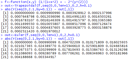
The screenshot above shows the result of solving the initial value problem $\begin{cases} \displaystyle y ' = {{1} \over {1 + x^2 }} - 2y^2 \\ y(0) = 0 \end{cases}$ with the trapezoidal method and the Euler method and comparing the errors against the true solution $\displaystyle Y = {{x } \over {1 + x^2}}$. Naturally, the error of the trapezoidal method is much smaller.

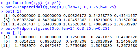
The screenshot above shows the result of solving the initial value problem $\begin{cases} \displaystyle y ' = x - y^2 \\ y(0) = 0 \end{cases}$ with the trapezoidal method and the midpoint method and comparing their numerical solutions. Seeing how its values oscillate toward the end, the midpoint method has a parasitic solution, whereas the trapezoidal method solves the problem stably and well.

Below is the code written in R. j is the number of times the iteration is repeated; if not entered separately, it just makes one guess with the Euler method and moves on.

Euler<-function(f,Y_0,a,b,h=10^(-3))
{
  Y <- t(Y_0)
  node <- seq(a,b,by=h)
  
  for(x in node)
  {
    Y<-rbind(Y,Y[length(Y[,1]),]+h*f(x,Y[length(Y[,1]),]))
  }
  
  return(Y)
}
 
Midpoint<-function(f,Y_0,a,b,h=10^(-3))
{
  Y <- t(Y_0)
  Y<-rbind(Y,Y[1,]+h*f(a,Y[1,]))
  node <- seq(a,b,by=h)
  
  for(x in node[-1])
  {
    Y<-rbind(Y,Y[length(Y[,1])-1,]+2*h*f(x,Y[length(Y[,1]),]))
  }
  
  return(Y)
}
 
Trapezoidal<-function(f,Y_0,a,b,h=10^(-3),j=0)
{
  Y <- t(Y_0)
  Y<-rbind(Y,Y[1,]+h*f(a,Y[1,]))
  node <- seq(a,b,by=h)
  
  for(x in node[-1])
  {
    Y_guess<-Y[length(Y[,1]),] + h* f(x,Y[length(Y[,1]),] )
    if(j>0)
    {
      for(temp in 1:j)
      {
        Y_guess<-Y[length(Y[,1]),]+(h/2)*( f(x,Y[length(Y[,1]),] )+ f(x+h,Y_guess) )
      }
    } else {"Wrong Iteration Number"}
    Y<-rbind(Y,Y[length(Y[,1]),]+(h/2)*( f(x,Y[length(Y[,1]),] )+ f(x+h,Y_guess) ))
  }
  
  return(Y)
}
 
Y<-function(x) {x / (1 + x^2)}
 
f<-function(x,y) {1/(1+x^2) + - 2*(y^(2))}
out<-Trapezoidal(f,seq(0,0,len=1),0,2,h=0.1)
abs(Y(seq(0,2.1,by=0.1)) - out[,1])
out<-Euler(f,seq(0,0,len=1),0,2,h=0.1)
abs(Y(seq(0,2.1,by=0.1)) - out[,1])
 
g<-function(x,y) {x-y^2}
out<-Trapezoidal(g,seq(0,0,len=1),0,3.25,h=0.25)
out[,1]
out<-Midpoint(g,seq(0,0,len=1),0,3.25,h=0.25)
out[,1]