An Easy Definition of the p-value or Significance Probability 📂Statistical Testing

An Easy Definition of the p-value or Significance Probability

Definition ¹

In hypothesis testing, the probability of rejecting the null hypothesis is called the p-value.

Explanation

You can think of it this way: if the p-value is smaller than the significance level, the null hypothesis is rejected. That the p-value is small under the null hypothesis can be understood as meaning that ’the evidence that the null hypothesis is wrong is that strong—too strong to be attributed to chance.'

Once terms like the power curve and the rejection region get attached to this, studying becomes harder, and no matter how hard you study, everyone gets confused when it comes down to null versus alternative. So it is more efficient to simply grasp the core concept properly. Those other things are worth a quick look when studying for midterms/finals, but on the long and distant road of statistics they are not that important.

In fact, at the undergraduate first- or second-year level, it is normal not to really get a feel for it no matter how much it is explained or how diligently you study. As you become an upperclassman and start dealing with actual analyses, you will become proficient with the p-value whether you like it or not. So even if you do not understand it well or find it confusing, there is no need to be too discouraged. The p-value is not something you learn but something you get used to.

The p-value is a probability.

That is, $0 \le p \le 1$. In nine out of ten cases where someone fails to understand this fact, they have not understood the definition of the p-value and instead think of it like some coefficient from another scientific field. Since hypothesis testing itself is not absolute after all, the p-value was introduced to express how reliable something is in probabilistic terms.

A lower p-value does not mean a stronger rejection

This is an important fact. At a significance level of $\alpha$, the null hypothesis is rejected as long as $p \le \alpha$.

One of the most common misconceptions about the p-value is the belief that a smaller p-value means the null hypothesis is rejected more strongly. Of course it is true that a smaller p-value allows the null hypothesis to be rejected even at a smaller significance level, but the ‘degree’ is irrelevant. Whether it is $0.001$, or $10^{-8}$, or some very small positive number $\varepsilon >0$, as long as it is smaller than the significance level, it is all the same rejection.

There is no good or bad in whether the null hypothesis is rejected

That is, there is no good or bad in the p-value being high or low. In this case, the students most curious about it are those who usually do not study and then cram at the last minute, but there is no answer to it. What is good or bad is judged by each person based on the result; the person handling the data has no need to make such a judgment and must not make one.

For example, the test statistic of the t-test or z-test becomes harder to occur toward both tails rather than the center, so it is rejected when its absolute value is large. In the Hosmer–Lemeshow goodness-of-fit test of logistic regression analysis, the test statistic follows the chi-squared distribution, and since being closer to $0$ means a better fit, it is rejected when the value is large.

If, in the two examples above, you got a sense of what was being rejected even though nothing was specifically designated as the null hypothesis, then you can consider yourself to have understood the p-value. At least in hypothesis testing, the null and alternative hypotheses are thus determined according to the distribution of the test statistic. Since the rejection region is set under the principle of maximizing the rejection region, this explanation of ‘an event that is hard to occur’ makes sense. If you imagine how the rejection region is determined at a given significance level, it will make sense.

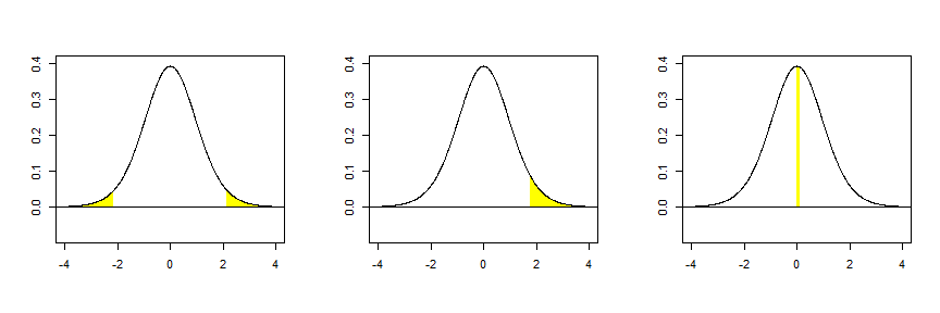
The rejection regions above all have the same area under the distribution function, but you can see that their lengths along the $x$-axis differ markedly. If asked to choose one of the three as the rejection region for a two-tailed test based on common sense, anyone would choose the first.

Code

Below is the R code used to draw the figure above.

win.graph(9,3)
 
par(mfrow=c(1,3))
plot(0,0,type='n',xlim=c(-4,4),ylim=c(-0.08,0.4),xlab=NA,ylab=NA)
 
polygon(c(seq(qt(0.975,14),5,0.01),qt(0.975,14)),
        c(dt(seq(qt(0.975,14),5,0.01),df=14),0),
        col='yelloW \',lty=0)
polygon(c(seq(-5,qt(0.025,14),0.01),qt(0.025,14)),
        c(dt(seq(-5,qt(0.025,14),0.01),df=14),0),
        col='yelloW \',lty=0)
abline(h=0)
lines(seq(-5,5,0.01),dt(seq(-5,5,0.01),df=14))
 
 
plot(0,0,type='n',xlim=c(-4,4),ylim=c(-0.08,0.4),xlab=NA,ylab=NA)
 
polygon(c(seq(qt(0.95,14),5,0.01),qt(0.95,14)),
        c(dt(seq(qt(0.95,14),5,0.01),df=14),0),
        col='yelloW \',lty=0)
abline(h=0)
lines(seq(-5,5,0.01),dt(seq(-5,5,0.01),df=14))
 
 
plot(0,0,type='n',xlim=c(-4,4),ylim=c(-0.08,0.4),xlab=NA,ylab=NA)
 
x<-c(seq(qt(0.50,14),qt(0.55,14),0.01))
y<-c(dt(seq(qt(0.50,14),qt(0.55,14),0.01),df=14))
x<-c(x[1],x,x[length(x)])
y<-c(0,y,0)
polygon(x,
        y,
        col='yelloW \',lty=0)
abline(h=0)
lines(seq(-5,5,0.01),dt(seq(-5,5,0.01),df=14))