Batch Normalization

Introduction¹

Suppose we are given training data $X = \left\{ \mathbf{x}_{1}, \cdots, \mathbf{x}_{N} \right\}$. Split it into mini-batches as $B = \left\{ B_{1}, \dots, B_{m} \right\}$ $(|B_{i}| = n)$, and write the $k$-th data point of $B_{i}$ as $\mathbf{x}_{i,k}$. For the $i$-th batch $B_{i}$, let $f$ be a suitable part of a neural network, let $H$ be the output dimension of that layer, and let the output of that layer for the $k$-th data point be $\mathbf{a}^{k} := f(\mathbf{x}_{i,k}) \in \mathbb{R}^{H}$. The matrix obtained by stacking these as rows is denoted by $\mathbf{A}$.

$$ \mathbf{A} = \begin{bmatrix} \left( \mathbf{a}^{1} \right)^{\mathsf{T}} \\ \left( \mathbf{a}^{2} \right)^{\mathsf{T}} \\ \vdots \\ \left( \mathbf{a}^{n} \right)^{\mathsf{T}} \end{bmatrix} = \begin{bmatrix} f(\mathbf{x}_{i,1})^{\mathsf{T}} \\ f(\mathbf{x}_{i,2})^{\mathsf{T}} \\ \vdots \\ f(\mathbf{x}_{i,n})^{\mathsf{T}} \end{bmatrix} \in \mathbb{R}^{n \times H} $$

In other words, $\mathbf{A}$ is the matrix whose $k$-th row is the output $\mathbf{a}^{k}$ for the $k$-th data point, and its $(k, j)$ entry $\left[ \mathbf{A} \right]_{kj} = \left[ \mathbf{a}^{k} \right]_{j}$ is the $j$-th component of the $k$-th data point.

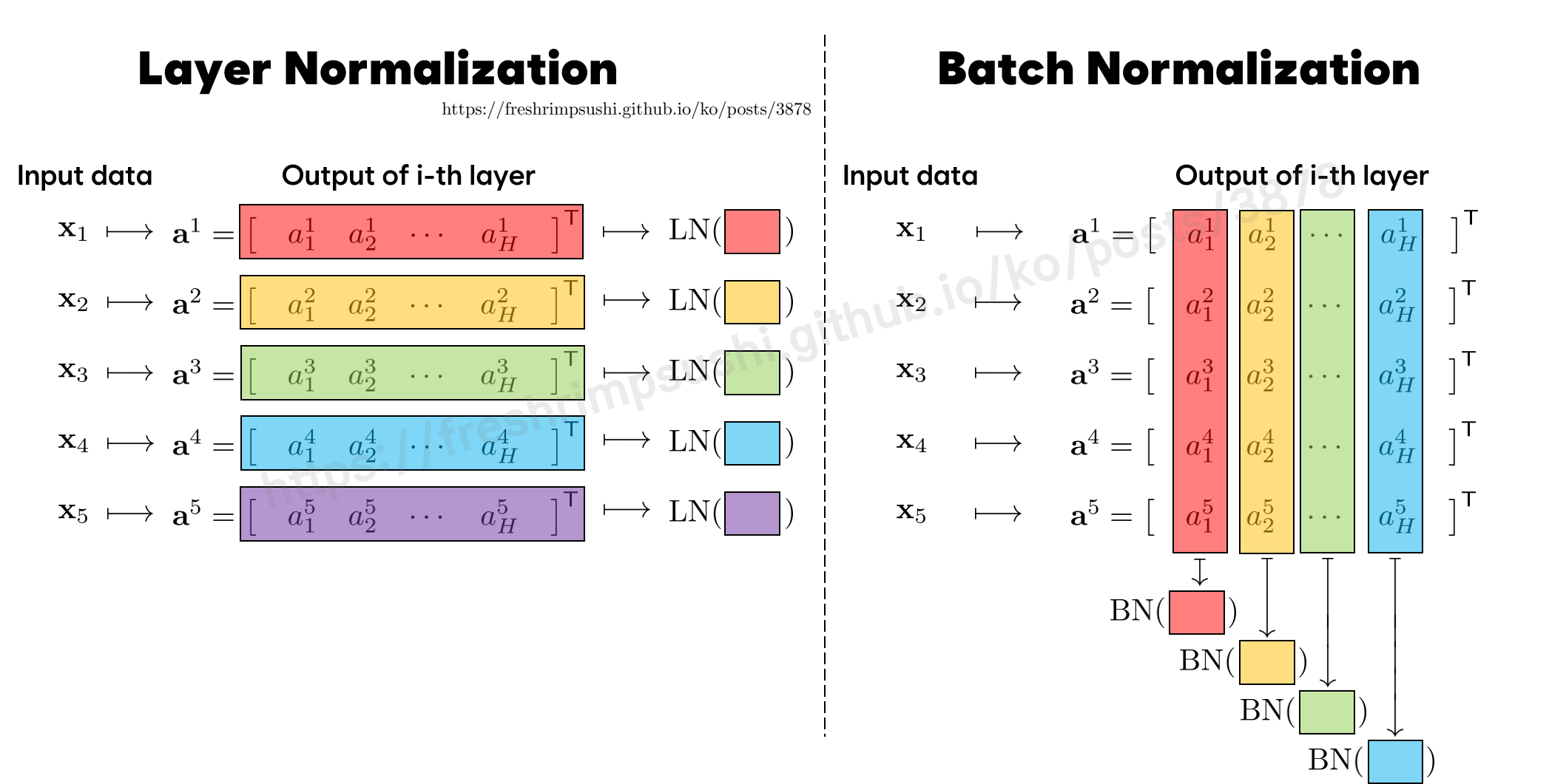
Let $\mathbf{1} \in \mathbb{R}^{n}$ be the vector whose entries are all $1$. The mean and variance computed along the batch direction for each component $j = 1, \dots, H$, that is, for each column of $\mathbf{A}$, are as follows.

$$ \mu_{j}(\mathbf{A}) := \frac{1}{n} \sum_{k=1}^{n} \left[ \mathbf{A} \right]_{kj} , \qquad \sigma_{j}^{2}(\mathbf{A}) := \frac{1}{n} \sum_{k=1}^{n} \left( \left[ \mathbf{A} \right]_{kj} - \mu_{j}(\mathbf{A}) \right)^{2} $$

Writing the vectors collecting these as $\boldsymbol{\mu}(\mathbf{A})$ and $\boldsymbol{\sigma}^{2}(\mathbf{A}) \in \mathbb{R}^{H}$, the mean is simply expressed as a matrix product, since it is the column-wise average of $\mathbf{A}$.

$$ \boldsymbol{\mu}(\mathbf{A}) = \frac{1}{n} \mathbf{A}^{\mathsf{T}} \mathbf{1} = \begin{bmatrix} \mu_{1}(\mathbf{A}) \\ \vdots \\ \mu_{H}(\mathbf{A}) \end{bmatrix} $$

The standard deviation is written as $\sigma_{j}(\mathbf{A}) := \sqrt{ \sigma_{j}^{2}(\mathbf{A}) }$.

Definition

For a scale $\boldsymbol{\gamma} \in \mathbb{R}^{H}$ and a shift $\boldsymbol{\beta} \in \mathbb{R}^{H}$, the following function $\operatorname{BN} : \mathbb{R}^{n \times H} \to \mathbb{R}^{n \times H}$ is called batch normalization.

$$ \operatorname{BN}(\mathbf{A}) := \begin{bmatrix} \gamma_{1} \dfrac{ \left[ \mathbf{A} \right]_{11} - \mu_{1}(\mathbf{A}) }{ \sigma_{1}(\mathbf{A}) } + \beta_{1} & \cdots & \gamma_{H} \dfrac{ \left[ \mathbf{A} \right]_{1H} - \mu_{H}(\mathbf{A}) }{ \sigma_{H}(\mathbf{A}) } + \beta_{H} \\ \vdots & \ddots & \vdots \\ \gamma_{1} \dfrac{ \left[ \mathbf{A} \right]_{n1} - \mu_{1}(\mathbf{A}) }{ \sigma_{1}(\mathbf{A}) } + \beta_{1} & \cdots & \gamma_{H} \dfrac{ \left[ \mathbf{A} \right]_{nH} - \mu_{H}(\mathbf{A}) }{ \sigma_{H}(\mathbf{A}) } + \beta_{H} \end{bmatrix} $$

That is, the entire $j$-th column is standardized by its mean $\mu_{j}(\mathbf{A})$ and standard deviation $\sigma_{j}(\mathbf{A})$, and then each column is multiplied by $\gamma_{j}$ and shifted by $\beta_{j}$.

Explanation

A transformation such as $Z = \dfrac{X - \mu}{\sigma}$ using the mean and standard deviation of $X$ is called standardization in statistics, while in machine learning it is called normalization. There is a strong tendency to call any transformation applied to data a normalization without distinction.

Meanwhile, just as multiplying a diagonal matrix on the left is the same as multiplying each entire row of the other matrix by the diagonal entries, multiplying a diagonal matrix on the right is the same as multiplying each entire column of the other matrix by the diagonal entries. Therefore, if we set the diagonal matrix $\mathbf{D}(\mathbf{A}) \in \mathbb{R}^{H \times H}$ as follows,

$$ \mathbf{D}(\mathbf{A}) := \diag \begin{bmatrix} \dfrac{\gamma_{1}}{\sigma_{1}(\mathbf{A})} & \cdots & \dfrac{\gamma_{H}}{\sigma_{H}(\mathbf{A})} \end{bmatrix} $$

the definition above can be expressed as follows.

$$ \operatorname{BN} (\mathbf{A}) = \left( \mathbf{A} - \mathbf{1} \boldsymbol{\mu}(\mathbf{A})^{\mathsf{T}} \right) \mathbf{D}(\mathbf{A}) + \mathbf{1} \boldsymbol{\beta}^{\mathsf{T}} $$

In actual implementations, a small $\epsilon > 0$ is added to the denominator to prevent division by $0$ when $\sigma_{j}(\mathbf{A}) = 0$. That is, the following $\mathbf{D}_{\epsilon}(\mathbf{A})$ is used instead of $\mathbf{D}(\mathbf{A})$.

$$ \mathbf{D}_{\epsilon}(\mathbf{A}) := \begin{bmatrix} \dfrac{\gamma_{1}}{\sqrt{\sigma_{1}^{2}(\mathbf{A}) + \epsilon}} & & \\ & \ddots & \\ & & \dfrac{\gamma_{H}}{\sqrt{\sigma_{H}^{2}(\mathbf{A}) + \epsilon}} \end{bmatrix} $$

$$ \operatorname{BN} (\mathbf{A}) = \left( \mathbf{A} - \mathbf{1} \boldsymbol{\mu}(\mathbf{A})^{\mathsf{T}} \right) \mathbf{D}_{\epsilon}(\mathbf{A}) + \mathbf{1} \boldsymbol{\beta}^{\mathsf{T}} $$

Written out componentwise, it is as follows.

$$ \left[ \operatorname{BN} (\mathbf{A}) \right]_{kj} = \gamma_{j} \dfrac{ \left[ \mathbf{A} \right]_{kj} - \mu_{j}(\mathbf{A}) }{ \sqrt{ \sigma_{j}^{2}(\mathbf{A}) + \epsilon } } + \beta_{j} $$

$\boldsymbol{\gamma}$ and $\boldsymbol{\beta}$ are learnable parameters. Since $\mathbf{D}(\mathbf{A})$ and $\boldsymbol{\mu}(\mathbf{A})$ depend on all rows of $\mathbf{A}$, the $k$-th row of $\operatorname{BN}(\mathbf{A})$ is not determined by $\mathbf{a}^{k}$ alone.

At inference time, it works differently. Since the output must not change depending on the input batch, a mean and variance fixed independently of the batch are needed in order to obtain a deterministic output. For this purpose, the means and variances of the mini-batches during training are computed as a moving average and used at inference time.

The paper that proposed it calls the phenomenon in which the distribution of inputs to each layer keeps changing as training progresses internal covariate shift, and explains that batch normalization reduces it and stabilizes training.

A visual comparison of how it works relative to layer normalization is shown below.