
Bidirectional Recurrent Neural Network
Introduction
The recurrent neural network (RNN) was devised to handle ordered data sequences such as time series. It works by having an encoder encode an input vector $\mathbf{x}_{i}$ and the hidden vector $\mathbf{h}_{i-1}$ of the immediately preceding state into a hidden vector $\mathbf{h}_{i}$, and a decoder decode the hidden vector $\mathbf{h}_{i}$ into an output vector $\mathbf{y}_{i}$. That is, $\mathbf{y}_{i}$ refers to the input vectors and hidden vectors only for all $t$ with $t \le i$. In other words, for some function $f$, it is expressed as follows.
$$ \begin{align*} \mathbf{y}_{1} &= f(\mathbf{x}_{1}, \mathbf{h}_{1}) \\ \mathbf{y}_{2} &= f(\mathbf{x}_{2}, \mathbf{h}_{2}, \mathbf{x}_{1}, \mathbf{h}_{1}) \\ &\vdots \\ \mathbf{y}_{t} &= f(\mathbf{x}_{t}, \mathbf{h}_{t}, \dots, \mathbf{x}_{1}, \mathbf{h}_{1}) \\ \end{align*} $$
However, in some situations $\mathbf{y}_{t}$ may need to refer to a vector $\mathbf{x}_{t+s}$ that has not yet been received as input. For example, consider the situation of translating the English sentence "I bought this book" into Korean. If we tokenize this sentence, it becomes the following sequence of input vectors.
$$ (\mathbf{x}_{1}, \mathbf{x}_{2}, \mathbf{x}_{3}, \mathbf{x}_{4}) = (\text{I}, \text{bought}, \text{this}, \text{book}) $$
The natural translation of this sentence is "나는 이 책을 샀다", and tokenizing it likewise gives the following output sequence.
$$ (\mathbf{y}_{1}, \mathbf{y}_{2}, \mathbf{y}_{3}, \mathbf{y}_{4}) = (\text{나는}, \text{이}, \text{책을}, \text{샀다}) $$
However, the third output token $\mathbf{y}_{3} = \text{책을}$ corresponds to the fourth input token $\mathbf{x}_{4} = \text{book}$, so in order to produce it correctly, we must refer to the future input $\mathbf{x}_{4}$ that has not yet been read. But as we saw earlier, the hidden state $\mathbf{h}_{t}$ of an RNN depends only on the inputs $\mathbf{x}_{1}, \dots, \mathbf{x}_{t}$ given up to now, so such a reference is structurally impossible. In other words, this structural limitation makes a degradation in performance unavoidable. What was proposed to overcome this limitation is the bidirectional recurrent neural network, a neural network that scans the input vector sequence in both the forward and backward directions so that the output at each time step can refer not only to past inputs but also to future inputs.
Definition1 2
Let $\overline{\sigma}$ be the function that applies the activation function $\sigma$ to each component of an input vector. That is, for a scalar function $\sigma : \mathbb{R} \to \mathbb{R}$, it is the vector function defined as follows.
$$ \overline{\sigma}(\mathbf{z}) = \begin{bmatrix} \sigma(z_{1}) \\ \sigma(z_{2}) \\ \vdots \\ \sigma(z_{m}) \end{bmatrix} \qquad \text{where } \mathbf{z} = \begin{bmatrix} z_{1} \\ z_{2} \\ \vdots \\ z_{m} \end{bmatrix} $$
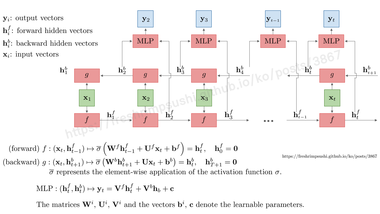
Suppose a sequence of input vectors $(\mathbf{x}_{1}, \mathbf{x}_{2}, \dots, \mathbf{x}_{T})$ $(\mathbf{x}_{t} \in \mathbb{R}^{n})$ is given. Let $\mathbf{W}^{f}, \mathbf{W}^{b} \in M^{m \times m}$, $\mathbf{U}^{f}, \mathbf{U}^{b} \in M^{m \times n}$ be weights, and let $\mathbf{b}^{f}, \mathbf{b}^{b} \in \mathbb{R}^{m}$ be biases. Define the forward hidden state $\mathbf{h}_{t}^{f} \in \mathbb{R}^{m}$ and the backward hidden state $\mathbf{h}_{t}^{b} \in \mathbb{R}^{m}$ by the following two recurrence relations.
$$ \begin{align*} \mathbf{h}_{t}^{f} &= \overline{\sigma}\left( \mathbf{W}^{f} \mathbf{h}_{t-1}^{f} + \mathbf{U}^{f} \mathbf{x}_{t} + \mathbf{b}^{f} \right), \qquad \mathbf{h}_{0}^{f} = \mathbf{0} \\ \mathbf{h}_{t}^{b} &= \overline{\sigma}\left( \mathbf{W}^{b} \mathbf{h}_{t+1}^{b} + \mathbf{U}^{b} \mathbf{x}_{t} + \mathbf{b}^{b} \right), \qquad \mathbf{h}_{T+1}^{b} = \mathbf{0} \end{align*} $$
The forward hidden state $\mathbf{h}_{t}^{f}$ is computed by increasing the time step from $t = 1$ to $T$, and the backward hidden state $\mathbf{h}_{t}^{b}$ is computed by decreasing the time step from $t = T$ to $1$.
The output $\mathbf{y}_{t} \in \mathbb{R}^{p}$ at each time step $t$ is obtained by passing the hidden states of the two directions through a fully connected layer respectively and adding them. If we let $\mathbf{V}^{f}, \mathbf{V}^{b} \in M^{p \times m}$ be weights and $\mathbf{c} \in \mathbb{R}^{p}$ be a bias, then a neural network that defines the output as follows is called a bidirectional recurrent neural network or BRNN.
$$ \mathbf{y}_{t} = \mathbf{V}^{f} \mathbf{h}_{t}^{f} + \mathbf{V}^{b} \mathbf{h}_{t}^{b} + \mathbf{c} $$
- The output formula $\mathbf{y}_{t} = \mathbf{V}^{f} \mathbf{h}_{t}^{f} + \mathbf{V}^{b} \mathbf{h}_{t}^{b} + \mathbf{c}$ presented in the definition is merely one example among the various ways of combining the hidden states of the two directions. For instance, in a classification problem one might apply a softmax so that the output can be interpreted as a probability, and in a regression problem one might pass it through an identity function or a nonlinear activation function. In the end, how one combines the hidden states of the two directions to produce the output is a matter of the field, use case, and implementation choice. One may understand the linear formula in this definition as the simplest representative form among them.
Explanation
Put simply, it uses for prediction the hidden states obtained by passing the vector sequences $\left\{ \mathbf{x}_{1}, \mathbf{x}_{2}, \dots, \mathbf{x}_{T} \right\}$ and $\left\{ \mathbf{x}_{T}, \mathbf{x}_{T-1}, \dots, \mathbf{x}_{1} \right\}$ through two separate RNNs.
In a basic recurrent neural network, the output $\mathbf{y}_{t}$ at time step $t$ depends only on the inputs $\mathbf{x}_{1}, \dots, \mathbf{x}_{t}$ up to now, through the hidden state $\mathbf{h}_{t}$. In contrast, a bidirectional recurrent neural network places two mutually independent recurrent neural networks: one compresses information in the direction of increasing $t$ $(t = 1 \to T)$, and the other compresses information in the direction of decreasing $t$ $(t = T \to 1)$. The hidden state produced by the former is the forward hidden state $\mathbf{h}_{t}^{f}$, and the hidden state produced by the latter is the backward hidden state $\mathbf{h}_{t}^{b}$.
Here, $\mathbf{h}_{t}^{f}$ summarizes and holds the past inputs $\mathbf{x}_{1}, \dots, \mathbf{x}_{t}$, while $\mathbf{h}_{t}^{b}$ summarizes and holds the future inputs $\mathbf{x}_{t}, \dots, \mathbf{x}_{T}$. Since the output $\mathbf{y}_{t}$ refers to both of these together, in the end the output at each time step is computed by looking at the entire input vector sequence. Even in a situation where $\mathbf{y}_{t}$ must refer to a later token $\mathbf{x}_{t+s}$ that has not yet been read, as in the translation example seen in the introduction, unlike an RNN the backward hidden state can compress and deliver that information.
Although it overcomes some of the drawbacks of the RNN, drawbacks unique to the BRNN still exist. Since it maintains separate parameters for the two directions, the number of parameters to be trained roughly doubles, and above all, to compute the backward hidden state, the entire input vector sequence must be given in advance. Therefore, a bidirectional recurrent neural network cannot be used for problems that must receive input in real time and immediately produce output, or for autoregressive generation that looks at previous outputs to generate the next input. Conversely, in tasks where the entire input vector sequence can be obtained all at once—such as the encoder of machine translation, part-of-speech tagging, named entity recognition, and speech recognition—the bidirectional structure can bring its advantages to bear.