
Knowledge Distillation
Definition
Knowledge distillation is a methodology that transfers the knowledge learned by a large, heavy model to a small, light model, so that the small model achieves performance comparable to the large model. Here, the large, heavy model is called the teacher, and the small, light model is called the student. It is a branch of model compression.
Explanation1 2
Neural networks with good performance are generally large. Models with hundreds of millions of parameters, or ensembles that average the predictions of several models, show excellent performance, but because they demand a great deal of computation and storage, they are difficult to deploy in resource-constrained environments such as mobile phones or embedded devices. The requirements of the model used for training and the model used for actual deployment are different. To bridge this gap, knowledge distillation transforms a model into a form suitable for deployment without losing its knowledge.
When we speak of transferring the knowledge of a heavy model to a small model, the first method that comes to mind is to use the answers the teacher model got right—that is, the correct labels—directly for training the student model. Letting the teacher model be $\operatorname{Teacher}(x)$ and the student model be $\operatorname{Student}(x; \theta)$, this means minimizing the difference between the outputs of the two models for an input $x$ over the entire dataset.
$$ \mathcal{L}(\theta) = \mathbb{E}_{x}\left[ \bigl\lVert \operatorname{Teacher}(x) - \operatorname{Student}(x; \theta) \bigr\rVert^{2} \right] $$
However, if we view the teacher’s output only as a single fixed prediction like this, it ends up being not much different from directly training the small model with the correct labels alone. The key to knowledge distillation lies in not identifying the knowledge held by a trained model with the concrete values of its parameters. If we look at knowledge more abstractly, it can be regarded as a mapping that carries input vectors to output vectors. A model that classifies multiple classes is trained to maximize the probability of the correct class, but as a byproduct it also assigns different probabilities to each of the incorrect classes.
For example, when classifying a photo of a BMW car, the probability of mistaking it for a garbage truck may be very small, yet it is still far greater than the probability of mistaking it for a carrot. The relative probabilities among the incorrect answers like this contain rich information about how the teacher model generalizes over the data. Knowledge distillation conveys precisely this information to the student model. Instead of telling it only the single correct answer, the entire probability distribution the teacher model assigned to each class is taken as the learning target. A probability distribution spread smoothly over all the classes like this is called a soft target, and the one-hot correct label, which is $1$ only for the correct answer and $0$ elsewhere, is called a hard target. Soft targets contain more information per training case than hard targets, and the variance of the gradient between cases is also smaller. Therefore, the student model can be trained with much less data and a higher learning rate than were used to train the original teacher model.
Temperature Softmax and the Loss Function
Neural networks for classification usually place a softmax layer at the end, converting the value computed for each class, the logit $z_{i}$, into a probability $q_{i}$.
$$ q_{i} = \dfrac{\exp(z_{i})}{\sum_{j} \exp(z_{j})} $$
In knowledge distillation, a temperature $T$ is introduced here, and the following modified softmax function is used.
$$ q_{i} = \dfrac{\exp(z_{i} / T)}{\sum_{j} \exp(z_{j} / T)} $$
When $T = 1$, it is the same as the usual softmax, and as $T$ increases, the probability distribution over the classes becomes softer.
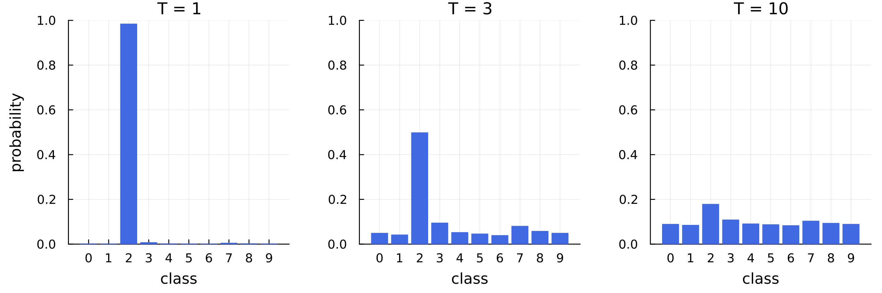
The figure above shows the result of applying different temperatures to the same logits. At $T = 1$, the probability is almost entirely concentrated on the single correct class, but as $T$ increases, the distribution spreads out more and more evenly, revealing the relative sizes of the small probabilities assigned to the incorrect classes.
Let the teacher model’s logits be $v_{i}$, the student model’s logits be $z_{i}$, and the soft probabilities each produces at temperature $T$ be $p_{i}$ and $q_{i}$, respectively. The student model is trained with a weighted mean of the following two loss functions.
$$ \mathcal{L} = \alpha T^{2}\mathcal{L}_{\text{soft}} + (1 - \alpha)\mathcal{L}_{\text{hard}} $$
- $\mathcal{L}_{\text{soft}}$ is the cross entropy between the teacher’s soft target $p_{i}$ and the student’s soft prediction $q_{i}$ at temperature $T$.
- $\mathcal{L}_{\text{hard}}$ is the cross entropy between the correct label and the student’s prediction at temperature $T = 1$.
- $\alpha$ is a weight that adjusts the balance between the two terms.
The temperature $T$ controls how soft the soft target is. In tasks like MNIST, where the teacher model gets the correct answer with very high confidence almost every time, most of the information about the learned function is hidden in the ratios of very small probabilities. (See the figure above.) For instance, some digit $2$ may be assigned a probability of $10^{-6}$ of being a $3$ and $10^{-9}$ of being a $7$; these values are valuable information telling us which $2$s resemble $3$s and which $2$s resemble $7$s. However, since the probabilities are so close to $0$, they have almost no effect on the usual cross entropy. Raising the temperature makes these small probabilities stand out, so that the similarity structure contained in them is reflected in training. In the figure above, when $T$ is raised from $1$ to $3$, the probability of being a $3$ grows from $10^{-6}$ to $0.1$, and the probability of being a $7$ grows from $10^{-9}$ to $0.01$, so the relative sizes between the two classes become far more apparent. However, if the temperature is set too high, such as $T = 10$, the distinction between the correct class and the incorrect classes becomes blurred.
Meanwhile, the magnitude of the gradients produced by the soft target shrinks in proportion to $1/T^{2}$. Therefore, when used together with the hard target, the soft term is multiplied by $T^{2}$ so that the relative contributions of the two terms remain roughly the same regardless of the temperature. This is why $T^{2}$ appears in front of $\mathcal{L}_{\text{soft}}$ in the loss function.
Generalization
Knowledge distillation can in fact be seen as a generalization of matching the student model’s logits to the teacher model’s logits. Let the probability predicted by the student model be $q_{i} = e^{z_{i}/T} / \sum_{j} e^{z_{j}/T}$, and the probability predicted by the teacher model be $p_{i} = e^{v_{i}/T} / \sum_{j} e^{v_{j}/T}$. Then the cross-entropy gradient contributing to the student’s logit $z_{i}$ for the $i$-th class is as follows.
$$ \begin{align*} \dfrac{\partial C}{\partial z_{i}} &= \dfrac{\partial}{\partial z_{i}} \left( -\sum_{k} p_{k} \log q_{k} \right) \\ &= \dfrac{\partial}{\partial z_{i}} \left[ -\sum_{k} p_{k} \left( \dfrac{z_{k}}{T} - \log \sum_{j} e^{z_{j}/T} \right) \right] \\ &= \dfrac{\partial}{\partial z_{i}} \left( -\dfrac{1}{T}\sum_{k} p_{k} z_{k} + \log \sum_{j} e^{z_{j}/T} \right) \\ &= -\dfrac{p_{i}}{T} + \dfrac{1}{T} \dfrac{e^{z_{i}/T}}{\sum_{j} e^{z_{j}/T}} \\ &= \dfrac{1}{T}\left( \dfrac{e^{z_{i}/T}}{\sum_{j} e^{z_{j}/T}} - p_{i} \right) \\ &= \dfrac{1}{T}\left( \dfrac{e^{z_{i}/T}}{\sum_{j} e^{z_{j}/T}} - \dfrac{e^{v_{i}/T}}{\sum_{j} e^{v_{j}/T}} \right) \end{align*} $$
If the temperature $T$ is sufficiently large compared to the magnitude of the logits, then by the Maclaurin series expansion of the exponential function, we can approximate $e^{x/T} \approx 1 + x/T$, and we obtain the following.
$$ \dfrac{\partial C}{\partial z_{i}} \approx \dfrac{1}{T}\left( \dfrac{1 + z_{i}/T}{N + \sum_{j} z_{j}/T} - \dfrac{1 + v_{i}/T}{N + \sum_{j} v_{j}/T} \right) $$
Here $N$ is the number of classes. If we assume the mean of the logits over all classes is $0$ $(\sum_{j} z_{j} = \sum_{j} v_{j} = 0)$, the above expression simplifies to the following.
$$ \dfrac{\partial C}{\partial z_{i}} \approx \dfrac{1}{N T^{2}}(z_{i} - v_{i}) $$
That is, in the high-temperature limit, knowledge distillation becomes equivalent to minimizing $\frac{1}{2}(z_{i} - v_{i})^{2}$, i.e., reducing the difference between the student’s and the teacher’s logits. Conversely, when the temperature is low, logits far below the mean (very negative ones) are almost entirely ignored. Since such logits are hardly constrained during the teacher model’s training and may be noise, ignoring them can actually help. When the student model is too small to hold all of the teacher’s knowledge, intermediate temperatures are known to work best.