📂Matrix Algebra

Least Squares Method

Definition¹

For a matrix $A \in \mathbb{C}^{m \times n}$ and a vector $\mathbf{b} \in \mathbb{C}^{m}$, suppose the linear system $A\mathbf{x} = \mathbf{b}$ is overdetermined or underdetermined. Then this system either has no solution or has infinitely many. In this case, consider the problem of minimizing the value of

$$ \left\| A \mathbf{x} - \mathbf{b} \right\|_{2} $$

This is called the Least Square problem (LSP). The solution $\mathbf{x}_{\ast}$ of this problem is called the least square solution.

$$ \mathbf{x}_{\ast} = \argmin \left\| A \mathbf{x} - \mathbf{b} \right\|_{2} $$

$A \mathbf{x} - \mathbf{b}$ is called the least square error vector, and $\left\| A \mathbf{x} - \mathbf{b} \right\|$ is called the least square error.

Explanation

It is unfortunate when a solution to an equation does not exist, but that does not mean we can give up on solving it altogether. In fact, most of the equations in this world that are hard to solve—those awaiting solutions from mathematicians at the frontier of academia—are precisely such problems. Studying methods to solve such problems even approximately is unquestionably valuable and useful, and the least squares method is one representative such method. It is actively used across many applied disciplines regardless of field, and in statistics in particular it is the theory that supports regression analysis, which is like the heart of the discipline. That the magnitude of $\left\| \mathbf{b} - A \mathbf{x} \right\|_{2}$ becomes minimal can be seen as the distance between $A \mathbf{x}$ and $\mathbf{b}$, that is, the error, becoming smaller by that much. For the orthogonal projection $P : \mathbb{C}^{m} \to \mathcal{C} (A)$, since

$$ \mathbf{b} = P \mathbf{b} + (I -P) \mathbf{b} $$

$$ P \mathbf{b} \in \mathcal{C} (A) $$

there exists some vector $\mathbf{x}_{\ast}$ such that $A \mathbf{x}_{\ast} = P \mathbf{b}$. Regarding this, if we express

$$ \left\| A \mathbf{x} - \mathbf{b} \right\|_{2} = \left\| A \mathbf{x} - P \mathbf{b} + P \mathbf{b} - \mathbf{b} \right\|_{2} $$

we can see that $( A \mathbf{x} - P \mathbf{b} ) \in \mathcal{C} (A)$ and $(I -P )\mathbf{b} \in \mathcal{N}(A)$ are orthogonal to each other. By the Pythagorean theorem,

$$ \left\| \mathbf{b} - A \mathbf{x} \right\|_{2}^{2} = \left\| A \mathbf{x} - P \mathbf{b} \right\|_{2}^{2} + \left\| (I -P )\mathbf{b} \right\|_{2}^{2} $$

and the case where $\left\| \mathbf{b} - A \mathbf{x} \right\|_{2}$ becomes smallest is $\mathbf{x} = \mathbf{x}_{\ast}$.

Meanwhile, from the properties of complementary projection, since $A \in \mathcal{C} (A)$ and $(I - P) \mathbf{b} \in \mathcal{C} (A)^{\perp}$,

$$ A^{\ast} (I - P) \mathbf{b} = A^{\ast} ( \mathbf{b} - A \mathbf{x}_{\ast} ) = 0 $$

Organizing this, since $A^{\ast} A \mathbf{x}_{\ast} = A^{\ast} \mathbf{b}$, the least squares method ultimately amounts to finding the solution $\mathbf{x}_{\ast}$ that satisfies the normal equation $A^{\ast} A \mathbf{x}_{\ast} = A^{\ast} \mathbf{b}$.

To understand it intuitively through a figure rather than through formulas, the following example will be helpful.

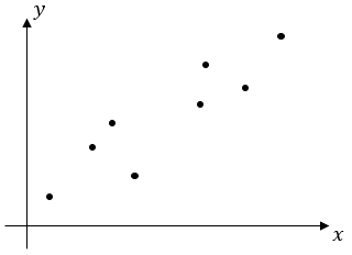
Suppose there is a problem of drawing a straight line that passes through all the points lying on a plane as shown above. Naturally, no straight line (solution) that serves as the answer to this problem exists, and we would have to look for a straight line (approximate solution) that at least passes through them somewhat closely.

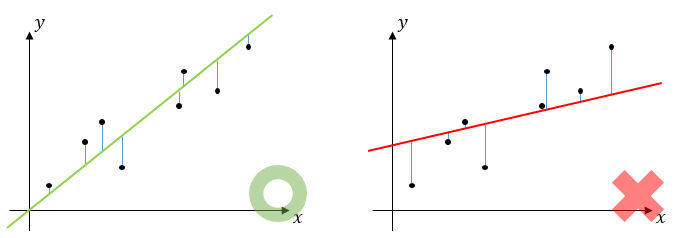
Comparing the green line and the red line as shown above, one can see at a glance that the left is more accurate than the right. The lengths of the lines drawn in blue represent the distances by which each point is separated when projected onto the straight line. In this problem, the least square solution is some straight line for which the sum of the squares of these distances is minimized.