📂Machine Learning

Importance Sampling

Overview¹

Introduction

In the standard normal distribution, the probability that the $z$ value is $4$ or greater is about $3.167 \times 10^{-5}$.

$$ \begin{equation} \int_{4}^{\infty} \dfrac{1}{\sqrt{2\pi}} e^{-z^{2}/2}dz \approx 3.167 \times 10^{-5} \end{equation} $$

The Julia code that computes this integral by Monte Carlo integration is as follows.

using Distributions

n = 50000                      # sample size
z₀ = 4.0

for i in 1:5
    z = rand(Normal(), n)      # n-samples drawn from a standard normal distribution 
    est_MC = sum(z .> z₀)/n    # estmiates using Monte Carlo
    println(est_MC)
end

4.0e-5
6.0e-5
0.0
4.0e-5
4.0e-5

If you try it about five times, the computed value is not close to the true value, and sometimes it is even computed as $0$. This inaccuracy arises because the tail of the standard normal distribution is too thin. When integrating on paper, no matter how thin the tail is, its contribution is included in the integral, but when sampling with a computer only a finite number of samples are handled, so events with too low a probability of occurring may not be included in the computation. Of course increasing $n$ will make it more accurate, but that is far too obvious a statement, and such a thing is not called a solution.

$$ \int f(x)p(x) dx = \int f(x)\dfrac{p(x)}{q(x)} q(x) dx = \int \left[ f(x)\dfrac{p(x)}{q(x)} \right] q(x) dx $$

Now let us consider the situation of computing the expectation of $f(X)$ for a random variable $X$ whose probability density function is $p$. This can be computed as in the left-hand side of the equation above, and here we may divide and multiply by some $q(x)$ and still get the same value. The right-hand side of the equation has the same value as the left-hand side, but its meaning becomes ’the expectation of $f(X)\dfrac{p(X)}{q(X)}$ for a random variable $X$ whose probability density function is $q$’. Here, if we choose $q$ to be a probability density function with a thicker tail than $p$, we can reduce the inaccuracy caused by events with too low a probability of occurring.

Definition

Let $X$ be a random variable whose probability density function is $p$. Let $q$ be another probability density function satisfying the following.

$$ \supp p \subset \supp q \qquad (\iff q\ne 0 \text{ if } p \ne 0) $$

Importance sampling is a method that computes the expectation $E_{p}[f(X)]$ of $f(X)$ as $E_{q}[f(X)\frac{p(X)}{q(X)}]$. Here $\supp$ is the support of a function.

$$ E_{p}[f] = \int f(x)p(x) dx = \int \left[ f(x)\dfrac{p(x)}{q(x)} \right] q(x) dx = E_{q}[fp/q] $$

Here $q$ is called the proposal distribution, and $w = \frac{p}{q}$ is called the importance weight.

Explanation

In other words, importance sampling is computing the Monte Carlo integral as follows.

$$ \dfrac{1}{n}\sum f(x_{i})\dfrac{p(x_{i})}{q(x_{i})}, X_{i} \sim q(x) \quad \left( \text{instead of } \dfrac{1}{n}\sum f(x_{i}), X_{i} \sim p(x) \right) $$

It is helpful to use it in the following ways.

• When the tail of $p(x)$ is too thin, as in the example in the buildup, take a distribution with a larger support as the proposal function.
• When it is difficult to sample from the distribution $p(x)$, take a distribution that is easy to sample from as the proposal function $q(x)$.

Since $q$ is multiplied as the denominator of $p$, $\supp q$ must contain $\supp p$.

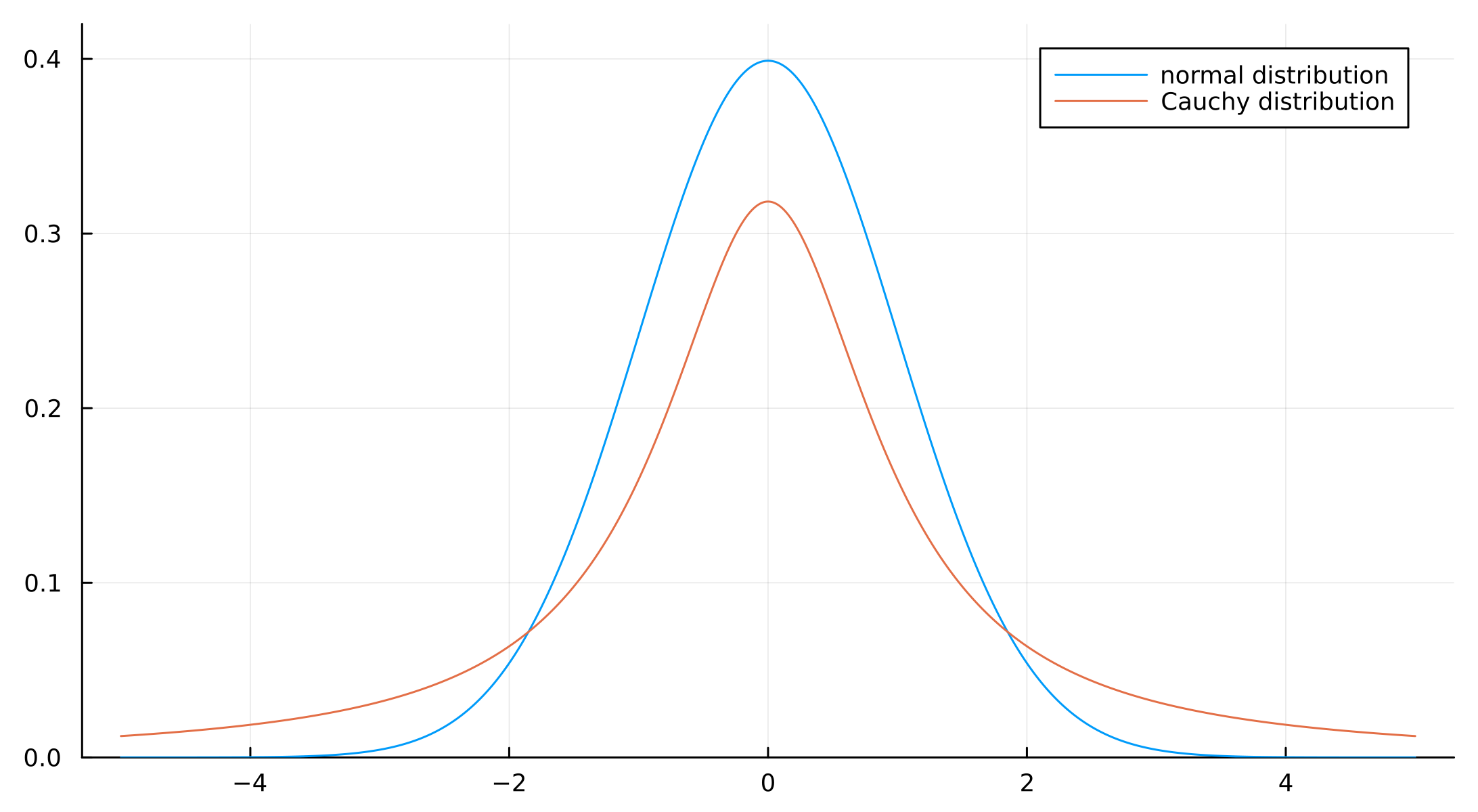
The result of recomputing the integral $(1)$ from the buildup by importance sampling, taking the Cauchy distribution as the proposal distribution, is as follows.

# Julia code

using Distributions

n = 50000                      # sample size
z₀ = 4.0

for i in 1:5
    z = rand(Cauchy(), n)                       # n-samples drawn from a Cauchy distribution 
    w = pdf.(Normal(), z) ./ pdf.(Cauchy(), z)
    est_IS = sum(w[z .> z₀])/n                  # estmiates using Importance Sampling
    println(est_IS)
end

3.0330744703037005e-5
3.1808448538011614e-5
3.049259883894785e-5
3.305423127141489e-5
3.1807695818207125e-5

Properties

Unbiased Estimator

$\dfrac{1}{n}\sum\limits f(x_{i})\dfrac{p(x_{i})}{q(x_{i})}$ is an unbiased estimator of $E_{p}[f(X)]$.

Proof

$$ \begin{align*} E_{q}\left[ \frac{1}{n}\sum_{i}^{n}f(X_{i})\dfrac{p(X_{i})}{q(X_{i})} \right] &= \frac{1}{n}\sum_{i}^{n} E_{q}\left[ f(X_{i})\dfrac{p(X_{i})}{q(X_{i})} \right] &\text{by linearity of $E$} \\ &= E_{q}\left[ f(X)\dfrac{p(X)}{q(X)} \right] \\ &= E_{p}\left[ f(X) \right] \end{align*} $$

■

Variance

The variance in importance sampling is

$$ \begin{align} \Var \left[ \frac{fp}{q} \right] &= E_{q}\left[ \left( \frac{fp}{q} \right)^{2} \right] - \left( E_{q}\left[ \frac{fp}{q} \right] \right)^{2} \\ &= \int \frac{f(x)^{2}p(x)^{2}}{q(x)} dx - \left( \int f(x)p(x) dx \right)^{2} \nonumber \end{align} $$

so, in order to have a finite variance, the following must hold.

$$ \int \frac{f(x)^{2}p(x)^{2}}{q(x)} dx \lt \infty $$

This means that $p(x)/q(x)$ must be bounded, which in turn means that the tail of $q(x)$ must be thicker than the tail of $p(x)$. The $q$ that minimizes the variance is as follows.

$$ q^{\ast} = \argmin\limits_{q} \Var [fp/q] = \frac{ \left| f(x) \right| p(x)}{ \int \left| f(x) \right| p(x) dx} $$

Proof

In $(2)$, although the second term appears to depend on $q$, since $E_{q}\left[ \frac{fp}{q} \right] = {\displaystyle \int} f(x)p(x)dx$, it is a value independent of $q$.

$$ \argmin\limits_{q} \Var [fp/q] = \argmin\limits_{q} E_{q}\left[ \left( \frac{fp}{q} \right)^{2} \right] $$

Jensen’s inequality

If a function $\phi$ is convex and twice differentiable on an open interval $I$, the expectation $\mu$ of a random variable $X$ exists, and $X \subset I $, then $$ \phi [ E(X) ] \le E [ \phi (X)] $$

Now, since a quadratic function is convex,

$$ \begin{align*} && \left( E_{q}\left[ \frac{fp}{q} \right] \right)^{2} &\le E_{q}\left[ \left( \frac{fp}{q} \right)^{2} \right] \\ \implies && \left( \int f(x)p(x) dx \right)^{2} &\le \int \frac{f(x)^{2} p(x)^{2}}{q(x)} dx \end{align*} $$

Here, equality holds when $q(x) = \frac{ \left| f(x) \right| p(x)}{ \int \left| f(x) \right| p(x) dx}$.

■