What is ReLU in Machine Learning? 📂Machine Learning

What is ReLU in Machine Learning?

Definition

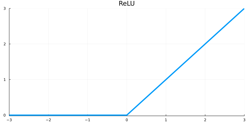
In machine learning, the following function is called the Rectified Linear Unit (ReLU).

$$ f(x) = x^{+} := \max \left\{ 0, x \right\} $$

Explanation

In electrical and electronic engineering, this is called the ramp function. For a description of the function itself or its properties (various ways of defining it, its derivative, etc.) rather than its viewpoint as an activation function in machine learning, refer to the ramp function document.

The name 'rectification' comes from rectification in electrical engineering, where a diode passes only the positive component of an alternating current signal. Since $\operatorname{ReLU}$ likewise passes the input through as is when it is positive and cuts it off to $0$ when it is negative, it operates just like a rectifier.

History

Rectifier-type activations appeared from the earliest days of neural network research. In 1969, Fukushima used an activation that cuts negative inputs off to $0$ in a multilayered neural network for visual feature extraction¹. The name ‘rectified linear unit’ originated from a paper presented by Nair and Hinton at ICML in 2010². They showed that replacing the hidden units of a restricted Boltzmann machine with rectified linear units improves performance. The following year, Glorot, Bordes, and Bengio showed that using rectifier activations instead of the sigmoid or hyperbolic tangent makes it possible to train deep neural networks well, even without the unsupervised pretraining that was regarded as essential for training deep neural networks at the time³.

Use as an Activation Function

The reasons $\operatorname{ReLU}$ is widely used as an activation function can be summarized as follows.

Mitigating vanishing gradients: The sigmoid function has a maximum derivative of $1/4$, and when the absolute value of the input is large, saturation occurs where the gradient approaches $0$; thus, stacking many layers inevitably causes vanishing gradients. In contrast, $\operatorname{ReLU}$ always has a derivative of $1$ in the positive region, so the gradient does not shrink as it passes through the layers, and thanks to this, much deeper neural networks can be trained.
Computational efficiency: Since it is done with a single comparison operation without computing an exponential function, both forward and backward propagation are much cheaper than the sigmoid family. Note that the fact that it is not differentiable at $0$ does not pose a problem in practice. In implementation, one can simply set the gradient at that point to $0$ or $1$.
Sparsity: A substantial portion of the output becomes exactly $0$, producing a sparse representation. Glorot et al. argue that this resembles the way actual neurons fire and is also advantageous for learning³.

Dying $\operatorname{ReLU}$ and Variants

Of course, there are drawbacks too. Since the gradient is exactly $0$ in the negative region, if the input of a certain neuron always becomes negative during training, that neuron is no longer updated. This is called the dying $\operatorname{ReLU}$ problem. To remedy this, $\operatorname{LeakyReLU}$, which leaves a small gradient $\alpha$ (usually $0.01$) in the negative region, was proposed⁴, and $\operatorname{PReLU}$, which learns the gradient $\alpha$ itself, followed⁵.

$$ \operatorname{LeakyReLU}(x) := \begin{cases} x & x \gt 0 \\ \alpha x & x \le 0 \end{cases} $$

Smooth variants that are differentiable even at $0$ include softplus and $\operatorname{GELU}$. $\operatorname{GELU}$ is defined as follows using the cumulative distribution function $\Phi$ of the standard normal distribution⁶, and is used as a standard in transformer-family models such as BERT and GPT.