📂Dynamical Systems

Bazykin Predator-Prey Model

Model¹

$$ \begin{align*} \dot{N_{1}}=& a N_{1} - b {\frac{ N_{1} N_{2} }{ N_{1} + N_{2} }} - \epsilon_{1} N_{1}^{2} \\ \dot{N_{2}}=& - c N_{2} + d {\frac{ N_{1} N_{2} }{ N_{1} + N_{2} }} - \epsilon_{2} N_{2}^{2} \end{align*} $$

Variables

• $N_{1} (t)$: the population size of the prey group $N_{1}$ at time $t$
• $N_{2} (t)$: the population size of the predator group $N_{2}$ at time $t$

Parameters

• $a$: natural growth rate of the prey
• $b$: rate of decrease of the prey due to the predator
• $c$: natural decay rate of the predator
• $d$: rate of increase of the predator due to the prey
• $\epsilon_{1}$: coefficient for competition among the prey
• $\epsilon_{2}$: coefficient for competition among the predators

Explanation

The Bazykin predator-prey model assumes that the prey and the predator, each of which follows logistic growth, obey the Lotka-Volterra predator-prey model, with the additional assumption that their interaction follows the Michaelis-Menten model as below. $$ {\frac{ N_{1} N_{2} }{ N_{1} + N_{2} }} $$

Bifurcation

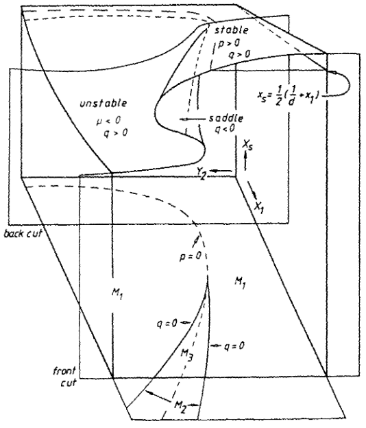
It can be regarded as a typical example that follows a cusp bifurcation.