📂Dynamical Systems

Bouali Attractor

Model¹

The following is the governing equation of the Bouali attractor.

$$ \begin{align*} \dot{x} =& x ( a - y ) + \alpha z \\ \dot{y} =& - y ( b - x^2 ) \\ \dot{z} =& - x ( c - s z ) - \beta x \end{align*} $$

Parameters

• $a = 4$
• $\alpha = 0.3$
• $b = 1$
• $c = 1.5$
• $\beta = 0.05$
• $s = 1$

Explanation

$$ \begin{align*} \dot{x} =& x ( a - y ) \\ \dot{y} =& - y ( b - x^2 ) \end{align*} $$

The Bouali attractor is a model obtained by adding a $z$-axis to a Lotka-Volterra model type system like the one above, thereby chaotifying it (chaotification). The form of $\dot{z}$ does not necessarily have to be exactly as shown; it only needs to have a natural oscillation and feed back into the prey $x$.

In fact, when one speaks of the Bouali equations, another similar form is also known, given below, with typical parameters $\alpha = 3$, $\beta = 2.2$, $\gamma = 1$, $\mu = 0.001$².

$$ \begin{align*} \dot{x} =& a x (1 - y) - \beta z \\ \dot{y} =& - \gamma y (x - 1) \\ \dot{z} =& \mu x \end{align*} $$

Attractor

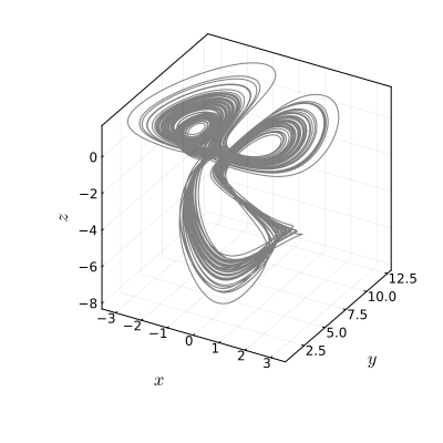
This is the strange attractor when $s = 1$. Compared to the Lorenz attractor, one gets the impression that something has sprouted and stretched out below the wings.

Bifurcation

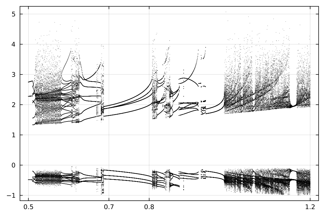
This is the bifurcation diagram drawn while varying $s$ from 0.5 to 1.2. Perhaps because the highest-order term is cubic, it shows a form as bizarre as that of the Aizawa attractor.

Code

The following is Julia code that simulates the Bouali attractor.

using DataFrames, DifferentialEquations, OrdinaryDiffEqLowOrderRK

function factory_bouali(s::Number; ic = [1.0, 1.0, 0.1], saveat = 0:1e-2:100)
      a,   α, b,   c,    β = (
      4, 0.3, 1, 1.5, 0.05)
    function sys(du, u, p, t)
        x, y, z = u
        s = p[1]

        du[1] = x*(a - y) + α*z
        du[2] = -y*(b - x^2)
        du[3] = -x*(c - s*z) - β*z
        return du
    end
    sol = solve(ODEProblem(sys, ic, (0, last(saveat)), [s]), RK4(), dt = saveat.step.hi, adaptive=false, maxiters = Inf)
    dsol = [sol.k[2][1] stack([solk[2] for solk in sol.k[2:end]])]
    matrix = [sol.t sol[:, :]' dsol']
    return matrix[sol.t .≥ first(saveat), :][1:end-1, :]
end
factory_bouali(T::Type, args...; kargs...) =
DataFrame(factory_bouali(args...; kargs...), ["t", "x", "y", "z", "dx", "dy", "dz"])

sol = factory_bouali(DataFrame, 1, ic = [2,1,0], saveat = 4500:1e-2:5000)
plot(sol.x, sol.y, sol.z, alpha = .5, color = :black, xlabel = L"x", ylabel = L"y", zlabel = L"z", size = [400, 400])

pm, pM = 0.5, 1.2; p0, p1 = 0.7, 0.8;
p_ = range(pm, pM, length = 1001)
bfcn = callbfcn("G:/BF/bouali/bfcnA.jld2")
@showprogress @threads for k in eachindex(p_)
    sol = factory_bouali(DataFrame, p_[k], saveat = 2500:1e-2:3000)
    bfcn[p_[k]] = sol.x[arglmax(sol.x)]
end
scatter(dict2bifurcation(bfcn)..., xticks = [pm, p0, p1, pM], ms = .5, ma = .5, msw = 0, color = :black); png("temp1")