📂Fluid Mechanics

Approximate Equations for a Fluid Layer on a Rotating Sphere

Model¹

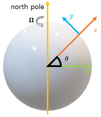
Consider a layer of fluid surrounding a sphere, for instance a celestial body, that completes one rotation per day so that its angular velocity is $\Omega = 2 \pi \text{rad / day}$. Here $x$ is the direction going from the eye into the plane of the screen, $y$ is the direction toward the north pole, and $z$ is the direction away from the center of the sphere. Let the angular velocity at the north pole be $\boldsymbol{\Omega} = \left( \Omega_{x} , \Omega_{y} , \Omega_{z} \right)$, and let the flow velocity at latitude $\theta$ be $(u, v, w)$. Usually $u$ is called the eastward, $v$ the northward, and $w$ the upward velocity. The governing equations for the flow velocity, written in the form of the Navier-Stokes equations, are as follows. $$ \begin{align*} {\frac{ D u }{ D t }} =& - {\frac{1}{\rho_{0}}} {\frac{ \partial P }{ \partial x }} + \nu_{\mathsf{h}} \left( {\frac{ \partial^{2} u }{ \partial x^{2} }} + {\frac{ \partial^{2} u }{ \partial y^{2} }} \right) + \nu_{\mathsf{v}} {\frac{ \partial^{2} u }{ \partial z^{2} }} + fv \\ {\frac{ D v }{ D t }} =& - {\frac{1}{\rho_{0}}} {\frac{ \partial P }{ \partial y }} + \nu_{\mathsf{h}} \left( {\frac{ \partial^{2} v }{ \partial x^{2} }} + {\frac{ \partial^{2} v }{ \partial y^{2} }} \right) + \nu_{\mathsf{v}} {\frac{ \partial^{2} v }{ \partial z^{2} }} - fu \\ {\frac{ D w }{ D t }} =& - {\frac{1}{\rho_{0}}} {\frac{ \partial P }{ \partial z }} + \nu_{\mathsf{h}} \left( {\frac{ \partial^{2} w }{ \partial x^{2} }} + {\frac{ \partial^{2} w }{ \partial y^{2} }} \right) + \nu_{\mathsf{v}} {\frac{ \partial^{2} w }{ \partial z^{2} }} - {\frac{ g \rho }{ \rho_{0} }} \end{align*} $$ Here $f := 2 \Omega \sin \theta$ is called the planetary vorticity or the Coriolis frequency. $\nu_{\mathsf{h}}$ and $\nu_{\mathsf{v}}$ are the eddy coefficients acting in the horizontal and vertical directions respectively, and $\rho$ and $\rho_{0}$ are the density and the reference density respectively. $P$ is the pressure, and $g$ is the gravitational acceleration.

Explanation

$$ \begin{align*} \Omega_{x} =& 0 \\ \Omega_{y} =& \Omega \cos \theta \\ \Omega_{z} =& \Omega \sin \theta \end{align*} $$ First, $\Omega$ at latitude $\theta$ is as above, and under the assumption $w \ll v$, the Coriolis force, being twice the cross product of $\Omega$ and the flow velocity, can be approximated as follows. $$ 2 \boldsymbol{\Omega} \times \begin{bmatrix} u \\ v \\ w \end{bmatrix} = \begin{bmatrix} - \left( 2 \Omega \sin \theta \right) v \\ \left( 2 \Omega \sin \theta \right) u \\ - \left( 2 \Omega \cos \theta \right) u \end{bmatrix} $$ Here the $z$-component $- \left( 2 \Omega \cos \theta \right) u$ is treated as $0$ under the assumption that it is almost negligible compared to gravity and pressure, and adding this force to the left-hand side of the Navier-Stokes equations yields the approximate equations.