📂Julia

How to Compute the Lyapunov Spectrum in Julia

Code

Let’s look at how to compute the Lyapunov spectrum in Julia. It is convenient because we use ChaosTools.jl, which is compatible with DifferentialEquations.jl, Julia’s standard differential equations package¹.

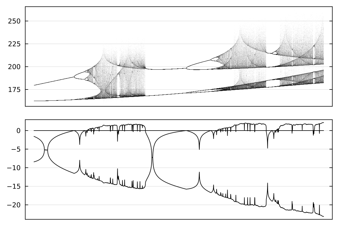
The figure above is the result of actually computing the Lyapunov spectrum of the Lorenz attractor over the ranges $\sigma \in [6, 15]$, $\rho \in [120, 150]$, $\beta \in [3, 5]$.

using DifferentialEquations, ChaosTools, ProgressMeter, Base.Threads, Plots

function sys(du, u, p, t)
    x, y, z = u; σ, ρ, β = p
    
    du[1] = σ*(y - x)
    du[2] = x*(ρ - z) - y
    du[3] = x*y - β*z
    return du
end

# sol = factory_lorenz63(DataFrame, [10, 28, 8/3])
# plot(sol.x, sol.y, sol.z, alpha = .5)

pm, pM = -2, 3; p0, p1 = 0, 1;
p_ = range(pm, pM, length = 2001)
σ_ = range(6, 15, length = 2001)
ρ_ = range(120, 150, length = 2001)
b_ = range(3, 5, length = 2001)
lpnv = callbfcn()
@showprogress @threads for k in eachindex(p_)
    lpnv[p_[k]] = lyapunovspectrum(CoupledODEs(sys, [100.0, 100, 100], [σ_[k], ρ_[k], b_[k]]), 100000)
end

• sys: Basically, you just define the differential equation in the form used in DifferentialEquations.jl. The official documentation uses SVector and so on, which is somewhat inconvenient, so I changed it to use ordinary arrays. The more complicated the equations, the more convenient this approach will be; if speed becomes critically important, it is better to refer to the originally provided guide.
• CoupledODEs: After the equation, the initial condition and the parameters are given.
• lyapunovspectrum: The function that computes the Lyapunov spectrum. It takes the number of iterations as its second argument, and the number must be sufficiently large to obtain accurate results.