📂Statistical Analysis

Neuromorphic Reservoir Computing

Algorithm¹

Reservoir computing: Suppose that the data up to $0 < t \leq T$ is divided at a constant time interval $\Delta t$, so that $K$ data points $\left\{ \left( \mathbf{u} \left( k \Delta t \right) , \mathbf{s} \left( k \Delta t \right) \right) \right\}_{k=1}^{K}$ are given. The predicted output vector $\hat{ \mathbf{s} }$ after $T$ is computed as follows. $$ \hat{ \mathbf{s} } (t + \Delta t) = W_{\text{out}} \left[ \left( 1 - \alpha \right) \mathbf{r} (t) + \alpha \tanh \left( A \mathbf{r} (t) + W_{\text{in}} \mathbf{u} (t) \right) \right] $$

• $\alpha \in [0, 1]$: leakage rate
• $A \in \mathbb{R}^{N \times N}$: adjacency matrix of the reservoir layer
• $W_{\text{in}} \in \mathbb{R}^{N \times M}$: input weight matrix
• $\tanh : \mathbb{R}^{N} \to \mathbb{R}^{N}$: vectorized hyperbolic tangent

A variant of reservoir computing, a technique inspired by the biological systems that describe the nervous system, is called neuromorphic reservoir computing.

Explanation

It is said that the neurons of the brain can be modeled as a map that has as parameters $b_{\text{ext}}$, $a_{\text{ext}}$, which are related to excitation (excitatory), and $b_{\text{inh}}$, $a_{\text{inh}}$, which are related to inhibition (inhibitory), as follows.

$$ \mathbf{x}_{t+1} = b_{\text{ext}} \tanh \left( a_{\text{ext}} \mathbf{x}_{t} \right) - b_{\text{inh}} \tanh \left( a_{\text{inh}} \mathbf{x}_{t} \right) $$

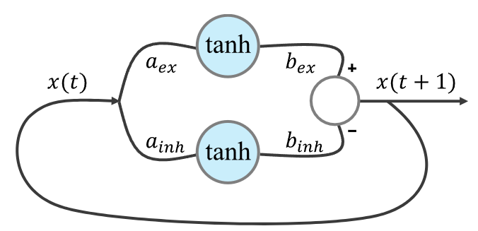
In conventional reservoir computing, a technique that mimics the dynamics of an actual system in this way is called physical reservoir computing. Unlike the usual echo state network (ESN) type of reservoir computing, which uses a single hyperbolic tangent function, neuromorphic reservoir computing builds the reservoir system using two $\tanh$ functions as follows. $$ \begin{align*} \mathbf{r} (t+1) =& b_{\text{ext}} \tanh \left( a_{\text{ext}} A \mathbf{r} (t) + W_{\text{in}} \mathbf{u} (t) \right) \\ & - b_{\text{inh}} \tanh \left( a_{\text{inh}} A \mathbf{r} (t) + W_{\text{in}} \mathbf{u} (t) \right) \end{align*} $$ Alternatively, there is also the following form, in which the influence of the input $\mathbf{u}(t)$ is taken outside of $\tanh$. $$ \mathbf{r} (t+1) = b_{\text{ext}} \tanh \left( a_{\text{ext}} A \mathbf{r} (t) \right) - b_{\text{inh}} \tanh \left( a_{\text{inh}} A \mathbf{r} (t) \right) + \mathbf{g} \left( W_{\text{in}} \mathbf{u} (t) \right) $$ Here $\mathbf{g}$ is a function meant to reflect intrinsic nonlinear characteristics, and the original paper gave as examples the identity function for comparison, $g(x) = \tanh(x)$, and the Gaussian kernel $g(x) = e^{-x^{2}}/2$. The paper claims that such an implementation of reservoir computing shows a level of performance comparable to that of conventional reservoir computing using thousands of nodes and much more data, even with a relatively small number of nodes ($N = 30$).

However, from the standpoint of someone who actually uses reservoir computing, the fact that hyperparameters such as $b_{\text{ext}}$, $a_{\text{ext}}$, $b_{\text{inh}}$, $a_{\text{inh}}$ increase in number, so that the burden of optimization grows larger, clearly acts as a drawback, and it is also bothersome that the relatively expensive $\tanh$ function has to be computed twice during the calculation. This will form some kind of trade-off against the gain of reducing the size of the network, but at least in terms of space complexity it seems certain to be advantageous.