📂Dynamical Systems

Aizawa Attractor

Model

$$ \begin{align*} \dot{x} =& (z - b)x - d y \\ \dot{y} =& d x + (z - b)y \\ \dot{z} =& c + a z - \frac{z^{3}}{3} - (x^{2} + y^{2})(1 + e z) + f z x^{3} \end{align*} $$

Parameters

• $a = 0.95$
• $b = 0.7$
• $c = 3.5$
• $d = 0.25$
• $e = 0.1$
• $f = 0.1$

Explanation

The Aizawa attractor is a dynamical system that exhibits complex chaos by including terms up to fourth order on the right-hand side, and it sometimes appears as a benchmark in techniques such as time series prediction.

However, while examining the origin and history of this system, I came to learn that Aizawa’s own paper does not exist, and that even in the literature where the Aizawa attractor does appear, the expressions of the equations differ from one to another^{1 2 3 4 5}. This is a rather peculiar situation for an attractor that has already gained fame and is being cited. In the main text I have gathered and organized the ordinary differential equations into what I consider to be the most common form among them.

Attractor

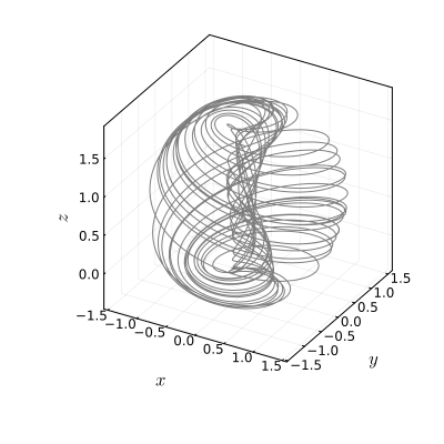
Even among strange attractors, it has a quite strange appearance. It basically takes the form of a sphere while having a structure that rotates and rises and falls along the $z$-axis.

Bifurcation

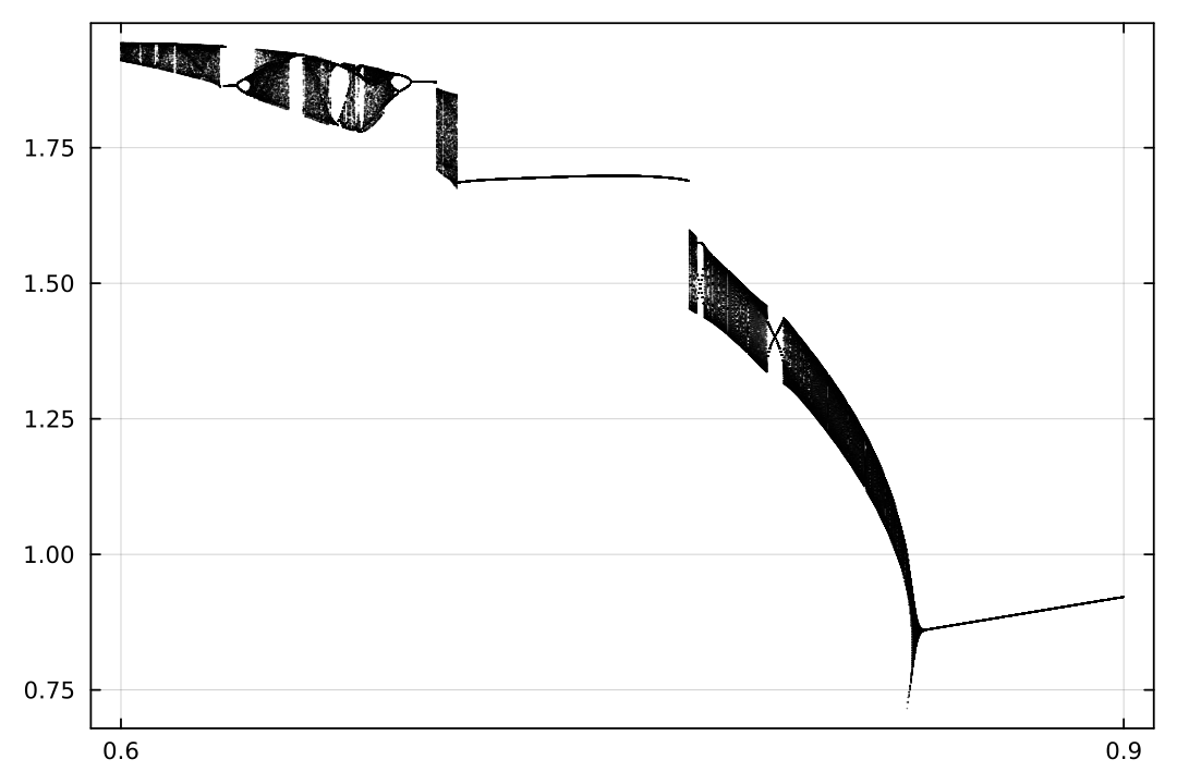
At least up until now, as I write this post, I have never seen a research result that mentions bifurcation related to the Aizawa attractor. The bifurcation diagram above records the maximum value of $z$ while varying $b$ from $0.6$ to $0.9$. As can be seen, it does not show the route to chaos that should commonly appear, and instead has a very bizarre form. I do not have time to study the Aizawa attractor right now, but someday I would like to dig deeply into this system.

Code

The following is Julia code that can simulate the Aizawa attractor.

using DataFrames, DifferentialEquations, OrdinaryDiffEqLowOrderRK

function factory_aizawa(b::Number; ic = [0.1, 0.1, 0.1], saveat = 0:1e-2:100)
      a,  c,   d,   e,  f = (
    .95, .6, 3.5, .25, .1)
    function sys(du, u, p, t)
        x, y, z = u
        b = p[1]

        du[1] = (z - b)*x - d*y
        du[2] = d*x + (z - b)*y
        du[3] = c + a*z - (z^3)/3 - (x^2 + y^2)*(1 + e*z) + f*z*x^3
        return du
    end
    sol = solve(ODEProblem(sys, ic, (0, last(saveat)), [b]), RK4(), dt = saveat.step.hi, adaptive=false, maxiters = 1e+7)
    matrix = Matrix([sol.t'; sol[:, :]; stack([sys(zeros(3), u, [b], 0) for u in sol.u])]')
    return matrix[sol.t .≥ first(saveat), :][1:end-1, :]
end
factory_aizawa(T::Type, args...; kargs...) =
DataFrame(factory_aizawa(args...; kargs...), ["t", "x", "y", "z", "dx", "dy", "dz"])

sol = factory_aizawa(DataFrame, 0.7)
plot(sol.x, sol.y, sol.z, alpha = .5, color = :black, xlabel = L"x", ylabel = L"y", zlabel = L"z", size = [400, 400])

pm, pM = 0.6, 0.9; p0, p1 = 0.72, 0.74;
p_ = range(pm, pM, length = 1001)
bfcn = callbfcn("G:/BF/aizawa/bfcnA.jld2")
@showprogress @threads for k in eachindex(p_)
    sol = factory_aizawa(DataFrame, p_[k], saveat = 0:1e-3:3000)
    z_ = sol.z[sol.t .≥ 2000]
    bfcn[p_[k]] = z_[arglmax(z_)]
end