📂Dynamical Systems

The Algae-Zooplankton Model as a Dynamical System

Model ¹

$$ \begin{align*} \dot{A} =& r A \left( 1 - \frac{A}{K} \right) - g Z \frac{A}{A + h_{A}} + i \left( K - A \right) \\ \dot{Z} =& e g Z \frac{A}{A + h_{A}} - m Z - F {\frac{ Z^{2} }{ Z + h_{Z} }} \end{align*} $$

Variables

• $A$: density of algae
• $Z$: density of zooplankton

Parameters

• $r = 0.5$: growth rate of algae
• $K = 6$: carrying capacity of algae
• $g = 0.4$: grazing rate of zooplankton
• $h_{A} = 0.6$: half-saturation constant of algae
• $i = 0.1$: inflow rate of algae
• $e = 0.6$: grazing efficiency of zooplankton
• $m = 0.15$: natural mortality rate of zooplankton
• $F$: loss due to the fish community
• $h_{Z} = 0.5$: half-saturation constant of zooplankton

Explanation

The algae-zooplankton model is a variant of the typical Lotka-Volterra predator-prey model, a mathematical model that describes the interaction between algae and zooplankton in water.

In the model above, each term has the following meaning.

• $\dot{A} = \cdots$
  • $r A \left( 1 - \frac{A}{K} \right)$: growth of algae, which follows logistic growth.
  • $g Z \frac{A}{A + h_{A}}$: grazing of algae by zooplankton, which follows a Holling type I functional response.
  • $i \left( K - A \right)$: inflow of algae, which is limited by the carrying capacity $K$ and follows the Euler migration model.
• $\dot{Z} = \cdots$
  • $e g Z \frac{A}{A + h_{A}}$: growth of zooplankton by algae, which is affected by the grazing efficiency $e \le 1$.
  • $m Z$: natural death of zooplankton.
  • $F {\frac{ Z^{2} }{ Z + h_{Z} }}$: the zooplankton eaten by fish, which follows a Holling type II functional response.

B-tipping

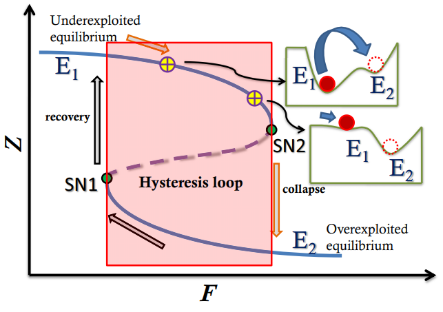
The given equation exhibits a bifurcation diagram similar to the one above as $F$ varies. There are two kinds of saddle-node bifurcations, so it shows hysteresis, and B-tipping naturally occurs.

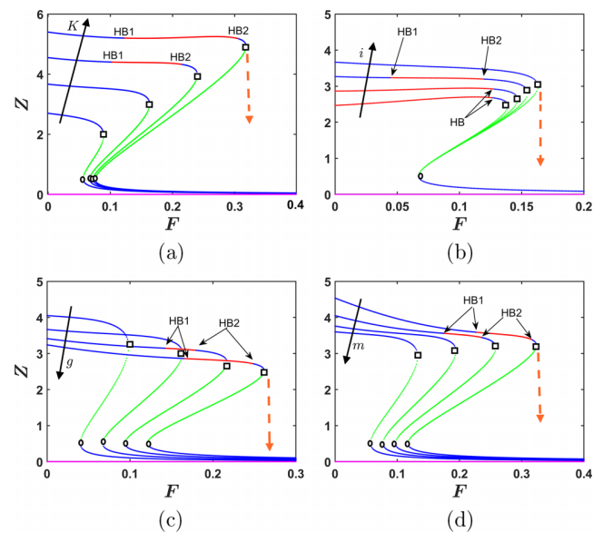
Such bifurcation diagrams appear differently in the figure above for (a) $K = 4, 6, 8, 10$, (b) $i = 0.025, 0.05, 0.075, 0.1$, (c) $g = 0.35, 0.40, 0.45, 0.50$, (d) $m = 0.10, 0.12, 0.14, 0.16$.

Code

The following is Julia code that can simulate the algae-zooplankton model.

using DataFrames, DifferentialEquations, OrdinaryDiffEqLowOrderRK

function factory_algaezooplankton(F::Number; ic = [5, 5], saveat = 0:1e-2:100)
      r, K,   g,  hA,   i,   e,    m,  hZ = (
    0.5, 6, 0.4, 0.6, 0.1, 0.6, 0.15, 0.5 )
    function sys(du, u, p, t)
        A,Z = u
        F = p[1]

        du[1] = r*A*(1 - frac(A,K)) - g*Z*frac(A, A + hA) + i*(K - A)
        du[2] = e*g*Z*frac(A, A + hA) - m*Z - F*frac(Z^2, Z^2 + hZ^2)
        return du
    end
    sol = solve(ODEProblem(sys, ic, (0, last(saveat)), [F]), RK4(), dt = saveat.step.hi, adaptive=false, maxiters = 1e+7)
    matrix = Matrix([sol.t'; sol[:, :]; stack([sys(zeros(2), u, [F], 0) for u in sol.u])]')
    return matrix[sol.t .≥ first(saveat), :][1:end-1, :]
end
factory_algaezooplankton(T::Type, args...; kargs...) =
DataFrame(factory_algaezooplankton(args...; kargs...), ["t", "A", "Z", "dA", "dZ"])