📂Dynamical Systems

The Plant-Pollinator Model as a Dynamical System

Model ¹

When the relationship between $N_{P}$ species of plants and $N_{A}$ species of pollinators is represented by a bipartite graph $\Gamma \left( N_{P}, N_{A} \right)$, the mutualism between plants and pollinators can be modeled through the following coupled dynamical system. $$ \begin{align*} \dot{P}_{i} =& P_{i} \left( \alpha_{i}^{P} - \sum_{l=1}^{N_{P}} \beta_{il}^{P} P_{l} + {\frac{ \sum_{j=1}^{N_{A}} \gamma_{ij}^{P} A_{j}} { 1 + h \sum_{j=1}^{N_{A}} \gamma_{ij}^{P} A_{j} }} \right) \\ \dot{A}_{j} =& A_{j} \left( \alpha_{j}^{A} - \kappa_{j} - \sum_{l=1}^{N_{A}} \beta_{jl}^{A} A_{l} + {\frac{ \sum_{i=1}^{N_{P}} \gamma_{ij}^{A} P_{i}} { 1 + h \sum_{i=1}^{N_{P}} \gamma_{ij}^{A} P_{i}}} \right) \end{align*} $$

Variables

• $P_{i}$ : abundance of the $i = 1 , \ldots , N_{P}$-th plant
• $A_{j}$ : abundance of the $j = 1 , \ldots , N_{A}$-th pollinator

Parameters

• $\alpha_{k}$ : intrinsic growth rate of the $k$-th species
• $\beta_{kl}$ : competition between the $k$-th species and the $l$-th species
• $\gamma_{ij}$ : interaction between the $i$-th plant and the $j$-th pollinator
• $\kappa_{j}$ : decline rate of the $j$-th pollinator

Explanation

In reality, the ecosystem formed by plants itself becomes the living ground on which pollinators survive, and pollinators play a key role in the reproduction of plants. The plant-pollinator model is a mathematical modeling of such interactions.

Looking at the equations, they seem complicated at first glance, but upon closer inspection they are nothing more than the Lotka-Volterra competition model with the sign of the competition term flipped to make it a cooperation term, and then its response set as Holling type 1. Competition within the same species, or within each group of plants and pollinators, follows logistic growth.

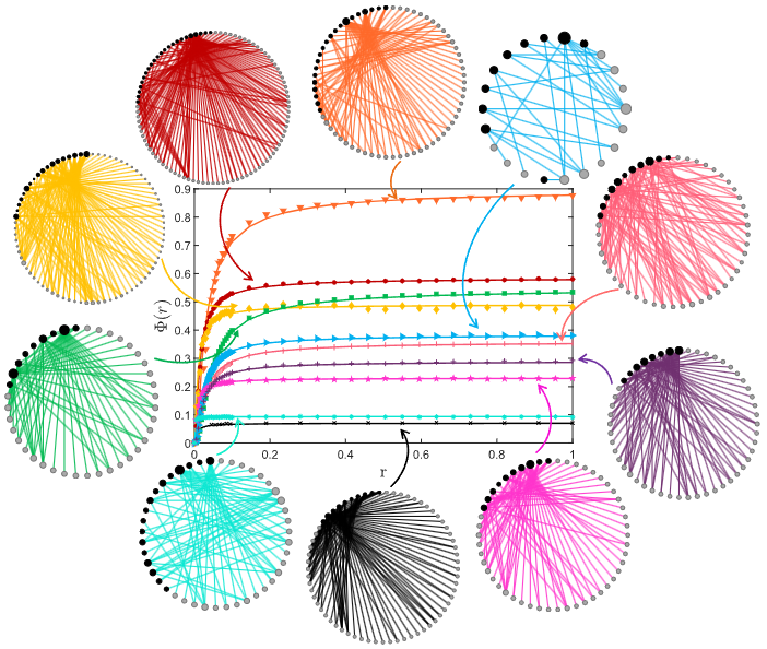
Here, the coefficients that make up the equations are based on real data provided by Web of Life. Looking at the figure above, we can see that the interaction between plants and pollinators differs depending on the type of data, and at the same time that there is no interaction among plants or among pollinators, following the structure of a bipartite graph.

R-tipping

A major topic in relation to climate change is precisely the fact that pollinators such as honeybees are disappearing. Accordingly, if we reflect the reality in which $\kappa_{j}$, which plays the role of reducing pollinators, increases steadily over time, this system becomes nonautonomous and can undergo R-tipping. $$ \dot{\kappa_{j}} = \begin{cases} r & , \text{if } \kappa_{\text{min}} < \kappa_{j} < \kappa_{\text{max}} \\ 0 & , \text{otherwise} \end{cases} $$ A large rate $r$ means that pollinators disappear that much faster, and with respect to this we can define the probability of undergoing $R$-tipping as follows. $$ \Phi (r) := B \exp \left[ - C \left( \kappa_{\text{min}} - \kappa_{\text{max}} \right) / r \right] $$ Here $C > 0$ is some constant, and $B > 0$ is a value related to the basin in which $A$ goes extinct, in other words the basin of the attractor with $A_{\infty} = 0$; it is obtained as the difference in area between the case $\kappa = \kappa_{\text{min}}$ and the case $\kappa = \kappa_{\text{max}}$, and in the case of the original high-dimensional system it is determined numerically.

Simplification

Rather than high-dimensional, an efficient 2-dimensional model can be expressed as follows.

$$ \begin{align*} \dot{P} =& P \left( \alpha - \beta P + {\frac{ \gamma^{P} A} { 1 + h \gamma^{P} A }} \right) \\ \dot{A} =& A \left( \alpha - \kappa - \beta A + {\frac{ \gamma^{A} P} { 1 + h \gamma^{A} P}} \right) \end{align*} $$

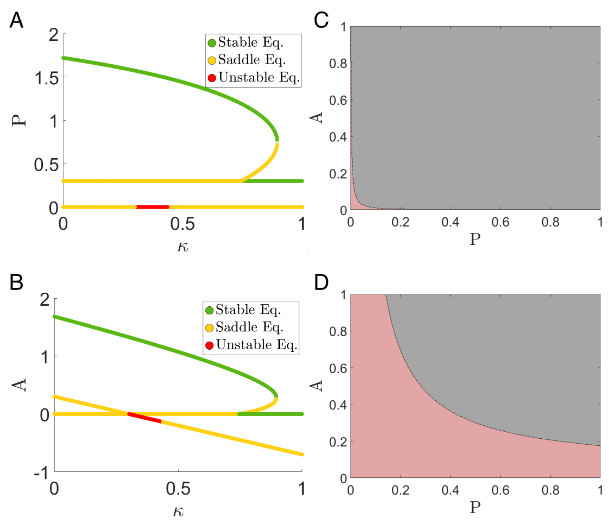
The explanation of $\Phi (r)$ in R-tipping was a bit difficult, so let us understand it by simplifying the essential content. In the network representation, the sky-blue (1 o’clock direction) data was constructed from the data called M_PL_036, and in this case the basins for $\kappa = \kappa_{\text{min}}$ and $\kappa = \kappa_{\text{max}}$ correspond respectively to $C$ and $D$ in the figure above. In the figure, the gray part is the basin for the fixed point where the pollinator $A$ coexists with $P$ without going extinct, and the red part is the basin for the fixed point where the pollinator $A$ goes extinct.

Now, thinking again about $\Phi (r)$, it is not that difficult: it is a matter of how the area of the basin concerning extinction changes as $\kappa_{\text{min}}$ changes to $\kappa_{\text{max}}$. That this difference is large means that the possibility of extinction is that much higher.

Code

The following is Julia code that can simulate the plant-pollinator model.

using DataFrames, DifferentialEquations, OrdinaryDiffEqLowOrderRK

function factory_pollinator(κ::Number; ic = [1.,1.], saveat = 0:1e-2:10)
      α, β,  _h,   γp,   γA = (
    0.3, 1, 0.4, 1.93, 1.77 )
    function sys(du, u, p, t)
        P,A = u
        κ = p[1]

        du[1] = P*(α - β*P + frac(γp*A, 1 + _h*γp*A))
        du[2] = A*(α - κ - β*A + frac(γA*P, 1 + _h*γA*P))
        return du
    end
    sol = solve(ODEProblem(sys, ic, (0, last(saveat)), [κ]), RK4(), dt = saveat.step.hi, adaptive=false, maxiters = 1e+7)
    matrix = Matrix([sol.t'; sol[:, :]; stack([sys(zeros(2), u, [κ], 0) for u in sol.u])]')
    return matrix[sol.t .≥ first(saveat), :][1:end-1, :]
end
factory_pollinator(T::Type, args...; kargs...) =
DataFrame(factory_pollinator(args...; kargs...), ["t", "P", "A", "dP", "dA"])