📂Dynamical Systems

Chua's Circuit

System ^{1 2}

$$ \begin{align*} \dot{x} =& \alpha (y - h(x)) \\ \dot{y} =& x - y + z \\ \dot{z} =& -\beta y \\ h(x) =& m_{1} x + \frac{1}{2} (m_{0} - m_{1}) \left( \left| x + 1 \right| - \left| x - 1 \right| \right) \end{align*} $$

Explanation

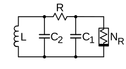
The $N_{R}$ in Chua’s circuit is the so-called Chua diode, a component that realizes the nonlinear resistance in the circuit. Although $h$ is not fixed by any strict rule, when a nonsmooth system is assumed, a form like the one above is usually used. When $h$ is defined in this way, the Chua circuit becomes a piecewise linear system.

For reference, Leon Ong Chua, who devised and studied this circuit, is an electrical engineer of Filipino origin, and Chua is written with the Chinese character 蔡. In our terms, it could also be called something like the Chae circuit.

Attractor

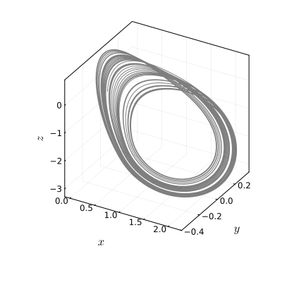
The Chua circuit has a chaotic attractor as follows.

Bifurcation Diagram

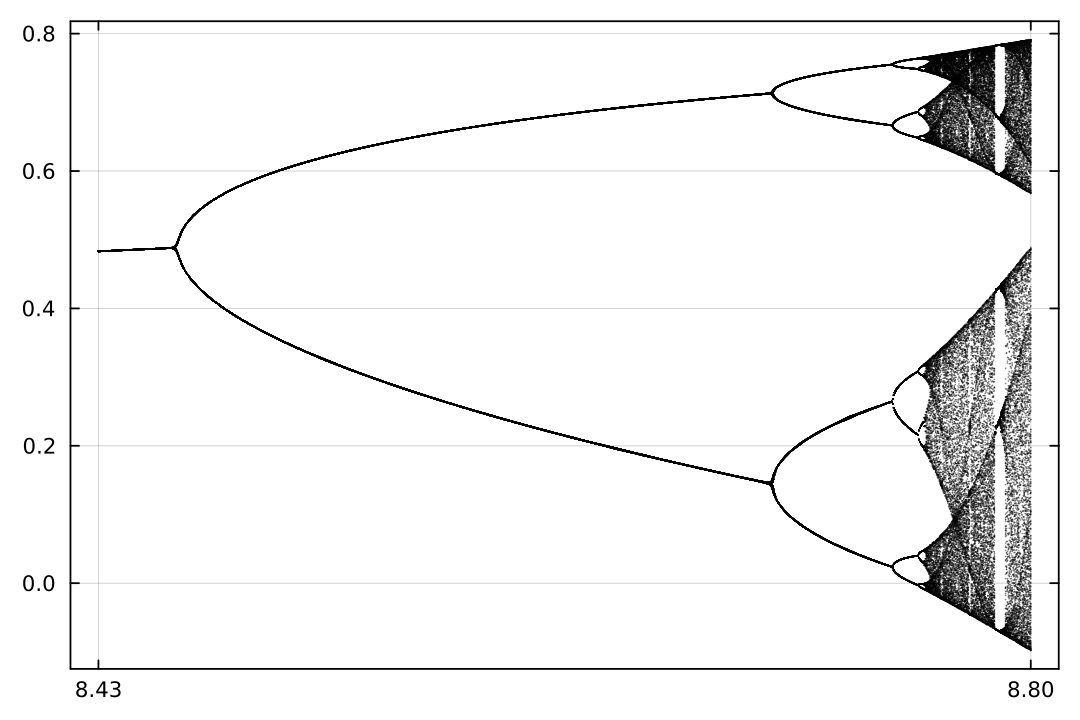
The following is the bifurcation diagram of the Chua circuit obtained by setting $\beta = 15$, $m_{0} = -1/7$, $m_{1} = 2/7$ and taking $\alpha$ as the bifurcation parameter.

Code

The following is Julia code that reproduces the attractor and bifurcation diagram of the Chua circuit.

using DataFrames, DifferentialEquations, OrdinaryDiffEqLowOrderRK

function factory_chua(α::Number; ic = [0.4, -0.2, 0.2], saveat = 0:1e-2:100)
     β,   m0,  m1 = (
    15, -1/7, 2/7)
    h(x) = m1*x + (m0 - m1)*(abs(x + 1) - abs(x - 1))/2
    function sys(du, u, p, t)
        x, y, z = u
        α = p[1]

        du[1] = α*(y - h(x))
        du[2] = x - y + z
        du[3] = -β*y
        return du
    end
    sol = solve(ODEProblem(sys, ic, (0, last(saveat)), [α]), RK4(), dt = saveat.step.hi, adaptive=false, maxiters = 1e+7)
    matrix = Matrix([sol.t'; sol[:, :]; stack([sys(zeros(3), u, [α], 0) for u in sol.u])]')
    return matrix[sol.t .≥ first(saveat), :][1:end-1, :]
end
factory_chua(T::Type, args...; kargs...) =
DataFrame(factory_chua(args...; kargs...), ["t", "x", "y", "z", "dx", "dy", "dz"])

sol = factory_chua(DataFrame, 8.8)
plot(sol.x, sol.y, sol.z, alpha = .5, color = :black, xlabel = L"x", ylabel = L"y", zlabel = L"z", size = [400, 400])

pm, pM = 8.430, 8.8; p0, p1 = 8.79, 8.80;
p_ = range(pm, pM, length = 1001)
bfcn = callbfcn("G:/BF/chua/bfcnA.jld2")
@showprogress @threads for k in eachindex(p_)
    sol = factory_chua(DataFrame, p_[k], saveat = 0:1e-3:3000)
    z_ = sol.z[sol.t .≥ 2000]
    bfcn[p_[k]] = z_[arglmax(z_)]
end
scatter(dict2bifurcation(bfcn)..., xticks = [pm, p0, p1, pM], ms = .5, ma = .5, msw = 0, color = :black); png("temp")