📂Julia

Solving Implicit Differential Equations and Differential-Algebraic Equations in Julia

Code

The following code recovers the Hastings–Powell system via implicit SINDy to build an implicit differential equation, and then solves it using Julia’s differential equation solving package as an example.

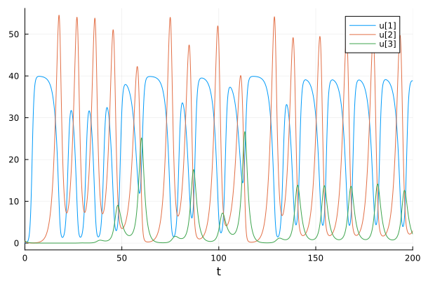
using Plots
import DifferentialEquations as DE
import Sundials
import DiffEqBase
function f2(out, du, u, p, t)
    out[1] = 2u[1] + 0.15u[1]^2 - 0.005u[1]^3 - 0.1u[1]*u[2] - 0.1u[1]*du[1] - du[1]
    out[2] = -u[2] - 0.1u[2]^2 + 0.1u[1]*u[2] - 0.15u[2]*u[3] - 0.015u[1]*u[2]*u[3] + 0.01u[1]*u[2]^2 - 0.1u[1]*du[2] - 0.1u[2]*du[2] - 0.01u[1]*u[2]*du[2] - du[2]
    out[3] = -0.7u[3] + 0.065u[2]*u[3] - 0.05u[2]*du[3] - du[3]
end
prob = DE.DAEProblem(f2, zeros(3), rand(3), (0, 200), differential_vars = [true, true, true])
sol = DE.solve(prob, Sundials.IDA(); initializealg = DiffEqBase.BrownFullBasicInit())
plot(sol)
plot(eachrow(stack(sol.u))...)

• Sundials provides IDA, a solver for solving implicit differential equations¹.
• DiffEqBase.BrownFullBasicInit() serves to reconcile the state and derivatives of the initial values.

As you can see, if you look closely at f2, you can observe that du—a term that would normally appear only on the left-hand side of an ordinary differential equation—also appears on the right-hand side. Even if it is not necessarily an implicit differential equation, you can write the differential equation so that the variable out becomes $0$. This means, for instance, that an expression such as the following is also possible.

$$ \begin{align*} f(\mathbf{x}, \dot{\mathbf{x}}) =& 0 \\ x_{1} + x_{2} = & 1 \end{align*} $$