Empirical Orthogonal Function Analysis: EOF 📂Statistical Analysis

Empirical Orthogonal Function Analysis: EOF

Definition

Principal component analysis applied to time series data is called Empirical Orthogonal Function analysis.

Explanation ¹ ²

EOF analysis is a statistical technique that seeks to summarize most of the original pattern using independent variables that explain the data dominantly but are relatively few in number and uncorrelated with one another. Intuitively speaking, it follows a philosophy somewhere between principal component analysis and the Fourier transform, and indeed its uses as well as its strengths and weaknesses can be seen as similar to those.

Since the actual implementation usually also uses singular value decomposition, it is PCA itself; the biggest reason PCA is not called PCA but is instead given the separate name EOF can be said to be a difference in field. In many cases EOF is related to the ocean and is applied to multivariate time series data covering vast sea areas.

In terms of Fourier analysis, EOF aims to express the trigonometric functions that serve as the basis as a linear combination of empirical functions $f_{k} : \mathbb{R} \to \mathbb{R}$ based on the data. This may be somewhat unfamiliar to mathematicians who are well versed in the general definition of a function, but it is worth considering that, from the standpoint of someone who majored in earth science, a function may be more familiar as the high-school-level function that outputs one number when one number is fed in.

The design matrix $X \in \mathbb{R}^{m \times n}$ is regarded as a panel dataset in which the $i = 1 , \cdots , m$-th timestep is recorded at $n$ points. As the result of the singular value decomposition of it, there will be matrices $U, \Sigma, V$, and the $j$-th column vector of $U$ immediately becomes the $j$-th EOF. The $j$-th singular value is interpreted, just as in PCA, as an indicator of the importance of the $j$-th EOF.

Example

This data is Sea Surface Temperature data collected at 150 points in the East Sea over five and a half years, and can be obtained from HYCOM.

alt text

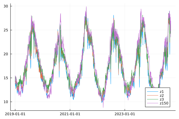
If the original data is as above, then the entire data is almost entirely explained by the first two EOFs as follows.

alt text

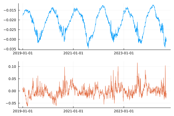
To obtain the $U$ that yields such a result, one simply needs to apply singular value decomposition to $X \in \mathbb{R}^{m \times 150}$. The following code is written in Julia, but the language does not matter much.

U, S, V = svd(Matrix(data))
plot(
    plot(U[:, 1]),
    plot(U[:, 2]),
)