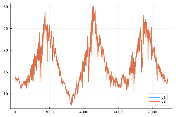
How to Compute the Inverse Fourier Transform Directly in Julia
Overview
To use the fast Fourier transform in Julia, you can use the FFTW.jl package. However, if you want to handle trigonometric functions directly instead of the already-implemented inverse Fourier transform ifft, you need to understand the Fourier series formally and be able to work with its coefficients.
Code
Slow Inverse Fourier Transform
Naturally, its speed is far slower than the optimized ifft, but since it is computed exactly the way we know the Fourier transform theoretically, it is intuitive and leaves plenty of room for intervention.
using DataFrames, FFTW, Plots

data = CSV.read("https://freshrimpsushi.github.io/ko/posts/2765/example.csv", DataFrame).x

Fs = 8
T = 120/8
fften = fft(data[1:round(Int64, Fs*T):end])

L = length(fften)
t_ = 1:L
a_ = 2real(fften[2:div(L,2)]) / L
b_ = -2imag(fften[2:div(L,2)]) / L

y = fill(real(fften[1]) / L, round(Int64, L))
for k in eachindex(a_)
    _sincos = sincospi.((2k/L)*t_)
    _sin = first.(_sincos)
    _cos = last.(_sincos)
    y .+= (a_[k] .* _cos) + (b_[k] .* _sin)
end
plot(data)
plot!(t_*(Fs*T), y, lw = 2)
Sampling Interval
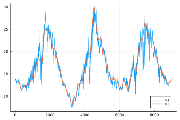
The following shows examples of computing the inverse Fourier transform while varying the sampling interval $T$.
$T = 120/8$
$T = 12/8$
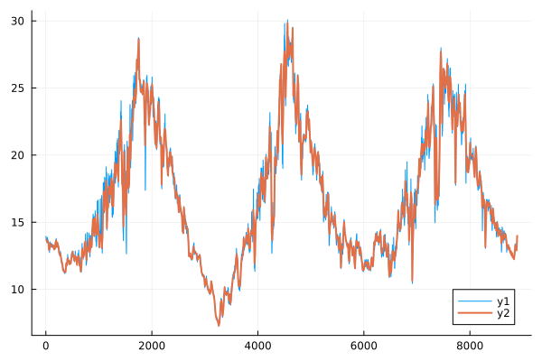
$T = 1/8$