📂Data Science

Sensitivity Analysis in Data Science

Definition ¹

Suppose we have a model (mostly in a regression problem) that has inputs and outputs. Assigning the output uncertainty of the model to the different sources of input uncertainty is called sensitivity analysis. In particular, when the model is expressed as a function of the form $f : \mathbb{R}^{n} \to \mathbb{R}$, quantifying the change of the output with respect to the $k = 1, \cdots , n$th input variable is sometimes called the sensitivity of the $k$th variable.

Explanation

The wording is difficult, but simply put, sensitivity analysis is examining ‘for which input the output changes the most’.

In Linear Regression Analysis

$$ f \left( x_{1} , \cdots , x_{n} \right) = \beta_{0} + \beta_{1} x_{1} + \cdots + \beta_{n} x_{n} $$ The linear regression analysis spoken of in classical statistics expresses the dependent variable as a linear combination of independent variables, as above. Here, the regression coefficient $\beta_{k}$ can itself be interpreted as the sensitivity of the $k$th input variable $x_{k}$.

Elementary Effect Method ^{2 3}

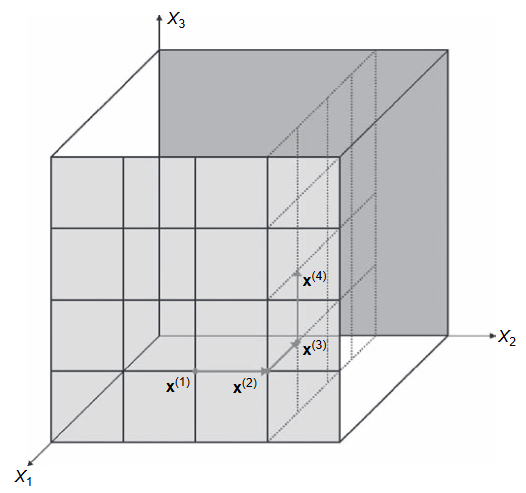
The elementary effect method, as shown above, maps the domain $\Omega$ of $f$ onto a hypercube, splits it into $p$ grids per dimension, and measures the change of the function value while passing through the grid points. For the $i$th independent variable, the elementary effect $EE_{i}$ is computed as follows. $$ EE_{i} = {\frac{ f \left( x_{1} , \cdots , x_{i} + \Delta_{i} , \cdots , x_{n} \right) - f \left( x_{1} , \cdots , x_{i} , \cdots , x_{n} \right) }{ \Delta_{i} }} $$ Here $\Delta_{i}$ is the amount of change of the $i$th independent variable. Observing the change while passing through grid points means that, since $2$ points are needed for each of the $n$ independent variables, $(n+1)$ points are needed by changing one per dimension, and the sequence obtained by listing those points is called a trajectory. The $EE_{i}$ obtained in this way is computed by repeating $r$ times until the mean converges, and finally the mean value $\mu_{i}$ of $EE_{i}$ is interpreted as the sensitivity of the $i$th independent variable. Meanwhile, Campolongo et al. also proposed $\mu_{i}^{\ast}$, which takes the absolute value of $EE_{i}$ and then averages it⁴. This method can prevent cases where, in the process of computing $\mu_{i}$, positive and negative values come out mixed together so that the mean value comes out low even for an important variable.

The elementary effect method has the advantage that it can compute the absolute sensitivity of input variables regardless of the form of $f$, but one must be careful that it is difficult to carry the interpretation all the way to the numerical value itself.

Implementation

The following is an implementation of the elementary effect method in Julia.

p = 4; p -= 1
Ω = extrema.(eachcol(data))
function elementary_effect(f, Ω, p = 4)
    p -= 1
    a_ = minimum.(Ω)
    b_ = maximum.(Ω)
    Δ_ = (b_ .- a_) ./ p

    x_ = [rand(0:p, n)]
    for k in 1:n
        x = deepcopy(x_[end])  
        if x[k] == 0
            x[k] = 1
        elseif x[k] == p
            x[k] -= 1
        else
            x[k] += rand([-1, 1])
        end
        push!(x_, x)
    end
    return abs.(diff(only.(f.([a_ + (Δ_ .* x) for x in x_]))) ./ Δ_)
end
EE = inv.(1:500)' .* cumsum(stack([elementary_effect(f, Ω, p) for _ in 1:500]), dims = 2)

Method Using the Range of Function Values ⁵

When using the range of function values, one first obtains the mean $\bar{x}_{1} , \cdots , \bar{x}_{n}$ for each independent variable from the data, and then computes all function values by changing only the $i$th independent variable, as follows. $$ Y_{i} = \left\{ f \left( \bar{x}_{1} , \cdots , x_{i} , \cdots , \bar{x}_{n} \right) : x_{i} \in X_{i} \right\} $$ Here $X_{i}$ refers to the set of all data obtained from the $i$th independent variable. Then the $i$th range $R_{i}$ is defined as follows. $$ R_{i} = \max Y_{i} - \min Y_{i} $$ The range cannot be negative, and finally the sensitivity for the $i$th independent variable is computed as a percentage as follows. $$ S_{i} = \frac{R_{i}}{\sum_{j=1}^{n} R_{j}} \times 100 \left( \% \right) $$

This method can be used even when the domain is not in the form of a hypercube, and it has the advantage that its interpretation is easy since it relatively evaluates for which input the output changes. However, one must be careful that, in that the mean $\bar{x}$ of the input variables is fixed, it cannot be said to consider the whole domain, and the $S_{i}$ itself is meaningless.

Implementation

The following is an implementation of the range-based method in Julia.

x̄ = mean.(eachcol(data[:, last(vrbl)]))
R_ = []
for k in 1:n
    X̄ = stack(fill(x̄, nrow(data)))
    X̄[k, :] = data[:, last(vrbl)][:, k]
    push!(R_, [extrema(only.(f.(eachcol(X̄))))...])
end
R = only.(diff.(R_))
R = R ./ sum(R)

Others

There are various methods⁶.