📂Topological Data Analysis

Derivation of Zomorodian's Algorithm

Overview

This post explains the derivation of the algorithm introduced in the paper ‘Computing Persistent Homology’ by Zomorodian and Carlsson¹. It takes a filtered complex built from an abstract simplicial complex and returns $\mathcal{P}$-intervals, computing persistent homology through matrix reduction while skipping the construction of the persistence module, which is difficult to handle on a computer.

Derivation

Part 0. Preliminary Investigation

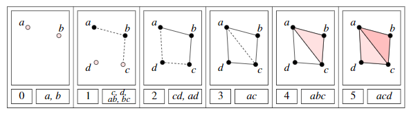
Before the full-fledged derivation of the algorithm, let us first look at what mathematical form the persistence complex depicted by the figure above actually takes. If this process is not firmly established, reading the paper will be extremely painful.

• First, call the number at the bottom $\deg$. This increases from $0$ to $5$ and forms a filtered complex as follows. $$ \left\{ a,b \right\} = K_{0} \subset K_{1} \subset K_{2} \subset K_{3} \subset K_{4} \subset \left( K_{4} \cup \left\{ acd \right\} \right) = K_{5} $$
• Regardless of $\deg$, $K$ is a $2$-simplex, and in the context of considering homology, it forms the following chain complex. $$ \mathsf{C}_{2} \overset{\partial_{2}}{\longrightarrow} \mathsf{C}_{1} \overset{\partial_{1}}{\longrightarrow} \mathsf{C}_{0} $$

The goal of the algorithm is to compute, as follows, the algebraic-topological information that such $\partial_{2}$ and $\partial_{1}$ give about the data—for instance, at which $\deg$ things like the Betti number $\beta_{k}$ are born and at which $\deg$ they disappear. $$ \begin{align*} L_{0} =& \left\{ \left( 0, \infty \right) , \left( 0,1 \right) , \left( 1,1 \right) , \left( 1,2 \right) \right\} \\ L_{1} =& \left\{ \left( 2,5 \right) , \left( 3,4 \right) \right\} \end{align*} $$

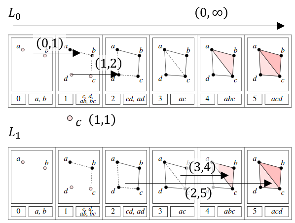
$L_{0}$ consists of the $\mathcal{P}$-intervals corresponding to $\beta_{0}$, that is, showing when components are born and disappear, and $L_{1}$ consists of the $\mathcal{P}$-intervals corresponding to $\beta_{1}$, that is, when the things called ‘holes’ in the space are born and disappear.

---

Part 1. $\partial_{1}$

In the paper, the authors claim that the computation for this is possible over any field, but let us simply look at what computation is carried out in the $\mathbb{Z}_{2} [t]$-module, which is a graded module. Now let us denote the homogeneous basis of $\mathsf{C}_{k}$ by $\left\{ e_{j} \right\}$ and the homogeneous basis of $\mathsf{C}_{k-1}$ by $\left\{ \hat{e}_{i} \right\}$. Here, homogeneous means that, viewing $\mathsf{C}_{k}$ as a graded module, there is only one term; that is, it is acceptable to regard it as a monomial form like $t^{4}$ rather than something like $t^{2} + t$.

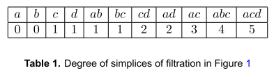
$$ \deg M_{k} (i,j) = \deg e_{j} - \deg \hat{e}_{i} $$ If you are somewhat familiar with homological algebra, you will now sense that we are going to construct the boundary matrix $M_{k}$ corresponding to $\partial_{k}$ according to the table and equation above, and go find its Smith normal form $\tilde{M}_{1}$. First, considering the case $k=1$, since we said earlier that the bases of the matrix are homogeneous, we can obtain the unique $M_{1}$ as follows.

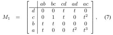
Constructing a matrix using bases in this way can be seen as reversing one of the roles of $\partial_{k}$, namely multiplying by $t^{n}$ (raising the degree in the graded module by taking a group action). To get a feel for it, let us compute directly just three times. $$ \begin{align*} \deg M_{1} (2,5) =& \deg ac - \deg c = 3 - 1 = 2 = \deg t^{2} \\ \deg M_{1} (4,5) =& \deg ac - \deg a = 3 - 0 = 3 = \deg t^{3} \\ \deg M_{1} (2,2) =& \deg bc - \deg c = 1 - 1 = 0 = \deg t^{0} = \deg 1 \end{align*} $$

As said before, if we now make its echelon form, in particular the column-echelon form, we get the following.

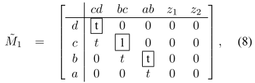
If we recall the linear algebra learned in undergraduate studies, the topmost nonzero entries in each column—the parts boxed in as in the figure—were called pivots. Here we introduce the following two lemmas.

• (1): The diagonal entries of the column-echelon form are the same as the diagonal entries of the Smith normal form.
• (2): If the pivot of row $i$ of $\tilde{M}_{k}$ is $\tilde{M}_{k} (i,j) = t^{n}$, then it corresponds to $\sum^{\deg \hat{e}_{i}} F[t] / t^{n}$ of the homology group $H_{k-1}$, and otherwise it corresponds to $\sum^{\deg \hat{e}_{i}} F[t]$ of $H_{k-1}$. This is equivalent to $L_{k-1}$ consisting of $\left( \deg \hat{e}_{i} , \deg \hat{e}_{i} + n \right)$ and $\left( \deg \hat{e}_{i} , \infty \right)$.

In other words,

• According to lemma (1), when computing persistent homology, no row operations are needed and only column operations are required.
• According to lemma (2), $L_{k-1}$ consists of $\left( \deg \hat{e}_{i} , \deg \hat{e}_{i} + n \right)$ and $\left( \deg \hat{e}_{i} , \infty \right)$.
  • The pivot of the first row is $t^{1}$ and $\deg d = 1$, so we get $(1,1+1)$.
  • The pivot of the second row is $t^{0}$ and $\deg c = 1$, so we get $(1,1+0)$.
  • The pivot of the third row is $t^{1}$ and $\deg b = 0$, so we get $(0,0+1)$.
  • The fourth row has no pivot and $\deg a = 0$, so we get $(0,\infty)$.

This exactly coincides with the $L_{0}$ mentioned before deriving the algorithm. $$ L_{0} = \left\{ \left( 0, \infty \right) , \left( 0,1 \right) , \left( 1,1 \right) , \left( 1,2 \right) \right\} $$

---

Part 2. $\partial_{2}$

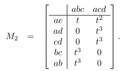
The matrix form $M_{2}$ of $\partial_{2}$ for obtaining $L_{1}$ is as above. However, here we can reduce the computation and proceed more easily with the following lemma.

• (3): To express $\partial_{k+1}$ with respect to the standard basis of $\mathsf{C}_{k+1}$ and $\mathsf{Z}_{k}$, we may simply remove from $M_{k+1}$ the rows corresponding to $\tilde{M}_{k}$.

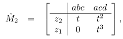
This sounds a bit difficult, but in our concrete situation right now, among the $1$-simplices $ab,bc,cd,ad,ac$ of $\tilde{M}_{1}$, only the pivots of $cd,bc,ab$ remain, so we may simply delete these from $M_{2}$. Intuitively, one may accept it to the extent that since these were already used in dimension $k$, there is no need to look at them in $k+1$. If we skip the process of directly obtaining the column-echelon form $\tilde{M}_{2}$ in this way and delete those three rows, we obtain the bottom-truncated $\check{M}_{2}$ as follows.

$$ \begin{align*} z_{2} =& ac - bc - ab \\ z_{1} =& ad - bc - cd - ab \end{align*} $$

Let us compute again according to lemma (2).

• The pivot of the first row is $t^{1}$ and $$ \deg z_{2} = \deg \left( ac - bc - ab \right) = \max \deg \left\{ ac , bc , ab \right\} = 3 $$ so we get $(3,3+1)$.
• The pivot of the second row is $t^{3}$ and $$ \deg z_{1} = \deg \left( ad - bc - cd - ab \right) = \max \deg \left\{ ad , bc , cd , ab \right\} = 2 $$ so we get $(2,2+3)$.

This exactly coincides with the $L_{1}$ mentioned before deriving the algorithm. $$ L_{1} = \left\{ \left( 2,5 \right) , \left( 3,4 \right) \right\} $$

Repeating this same process as many times as the dimension $\dim K$ of the complex $K$ yields the algorithm we wanted. It will be a little less confusing to think of the left-right size of the matrix as following $\partial_{k}$, and its entries as following $\deg$.

■

Meanwhile, the fact that column operations alone suffice in lemma (1) also means that there is no particular reason to insist on the matrix representation as we have seen in the derivation so far. Moreover, according to lemma (3), there is included an efficient procedure of boldly discarding rows for the parts that have ‘already been computed in the past’, and for this we need capabilities such as ‘marking’ non-pivot columns. As a result, the pseudocode of the actual algorithm is explained not by using the matrix directly, but by using a slightly higher-level data type, something like a dictionary or a dataframe. This is quite bewildering and difficult when you experience it firsthand.

Implementation

• Implementation of Zomorodian’s Algorithm: We introduce an implementation that transcribes the paper’s pseudocode almost literally, through the Julia language, which anyone working in the sciences can read comfortably.