Malthusian Growth Model: Ideal Population Growth
Model
$$ \dot{N} = rN $$
Variables
- $N(t)$: represents the population size of the group at time $t$.
Parameters
- $r \in \mathbb{R}$ : the intrinsic Rate of Increase; if it is greater than $0$ the population grows, and if it is less than $0$ it declines. It is sometimes defined as the difference $r:=b-d$ between the birth rate $b$ and the death rate $d$.
Explanation
population dynamics is the first gateway through which dynamics leads into mathematical biology, a mathematical approach to topics such as the population size of a group or the coexistence of species. The Malthusian growth model is the simplest of such growth models, and the population size of a species that can reproduce ideally (without any interference) can be expressed by a simple ordinary differential equation. Since the given equation is a separable first-order differential equation, its solution is obtained, for the initial population $N_{0}$, as
$$ N(t) = N_{0} e^{rt} $$
and since an exponential function appears in the equation, the expression that it increases exponentially fits perfectly, so it is also called the exponential Growth model. The name Malthusian growth model is taken from the name of Thomas Robert Malthus, the author of An Essay on the Principle of Population.
At first glance one might wonder where a population model could be useful, but more advanced models are actually used in the bio field in connection with the number of bacteria, viruses, or specific base sequences, and by discarding the meaning of population size and approaching it as a ‘moving quantitative variable’ itself, it also becomes the foundation of many applied models. For example, Gordon Moore, the co-founder of Intel, said that “the performance of semiconductor integrated circuits doubles every two years,” which literally means exponential growth and is now called Moore’s law . This does not mean that Moore said it by applying the Malthusian growth model, but rather that the phenomenon of growth is important because it is generally explained in this way. Even outside the bio field, this thing called growth can be applied to customers who use a service or the principal-and-interest total of a risk-free asset in economics/management, and conversely the radioactive decay of atomic nuclei can be viewed as the reverse growth of the number of atomic nuclei.
Derivation
To model the growth of a group, it is good to imagine bacteria that reproduce by binary fission. The rate at which the population increases will inevitably be proportional not only to each individual’s growth rate but also to the total population size itself. For example, if we think of a culture dish $A$ with $10$ bacteria and a culture dish $B$ with $20$ bacteria, then when the population has doubled after the same amount of time, $A$ will have $20$ and $B$ will have $40$. In other words, since
$$ (N = 10 \text{일 때의 증가량}) = 10 \\ (N = 20 \text{일 때의 증가량}) = 20 $$
holds, expressing it using the letter $N$,
$$ (N \text{의 증가량}) = N $$
we can assume that this holds. Here, if we modify the equation so that the growth rate can be taken into account, then for some real number $r \in \mathbb{R}$ it can be expressed as
$$ (N \text{의 변화량}) = rN $$
If $r>0$, the change in population is positive, so the population increases, and if $r<0$, the change is negative, so the population will decrease over time. Now, to express this change as a formula rather than in words, we need differentiation. Since the degree to which $N$ changes at time $t$ is $dN / dt$, modifying the left-hand side we obtain the following.
$$ {{dN} \over {dt}} = r N $$
■
Limitations
The word differential equation, or its formulas, may seem intimidating, but once you take them apart one by one you will be able to agree that they all start from a derivation based on common-sense premises. However, belying the explanation that they are common-sense premises, the biggest problem with this model is that it does not reflect reality at all. It may be appropriate as the first example in a textbook because it is easy and simple, but with this alone no practical application is possible at all.
The growth of an actual population inevitably faces a limitation also called the malthusian Trap. Continuing to think about the example of bacteria in a culture dish, within the small system of a culture dish, they are not provided with enough nutrients to grow and reproduce forever, and that space itself is finite. Eventually, from some moment on, the growth trend will bend, and the ideal growth will come to a halt.
Since this model is the simplest, it is rarely used to actually fit real population sizes; instead, it either carries meaning only as a first-order term in itself, or various models are used to overcome its unrealism. For instance, one could consider methods such as reflecting death, or having multiple species compete with one another.
Visual Understanding
Let us implement the Malthusian growth model with an agent-based simulation and understand it visually.
Actions
(Every agent, every turn)
- Reproduction: with probability
b, creates a new agent at its own position. - Death: with probability
d, is removed from the simulation.
b # 번식률
d # 사망률
replicated = (rand(N) .< b) # 번식 판정
new\_coordinate = coordinate[replicated,:]
coordinate = coordinate[rand(N) .> d,:] # 사망 판정
coordinate = cat(coordinate, new\_coordinate, dims = 1);
We used only the simple actions of an agent’s reproduction and death, and it is enough to check how the system changes as the parameter corresponding to the intrinsic growth rate $r$ in the system is varied.
What must be noted is that the reproduction probability b used in the simulation and the system’s birth rate $b$, and the death probability d and the system’s death rate $d$, are usually not the same. Since they do not exactly match the autonomous system expressed by the differential equation, the fitting to the simulation was done by intuitively finding parameters that are reasonably appropriate.
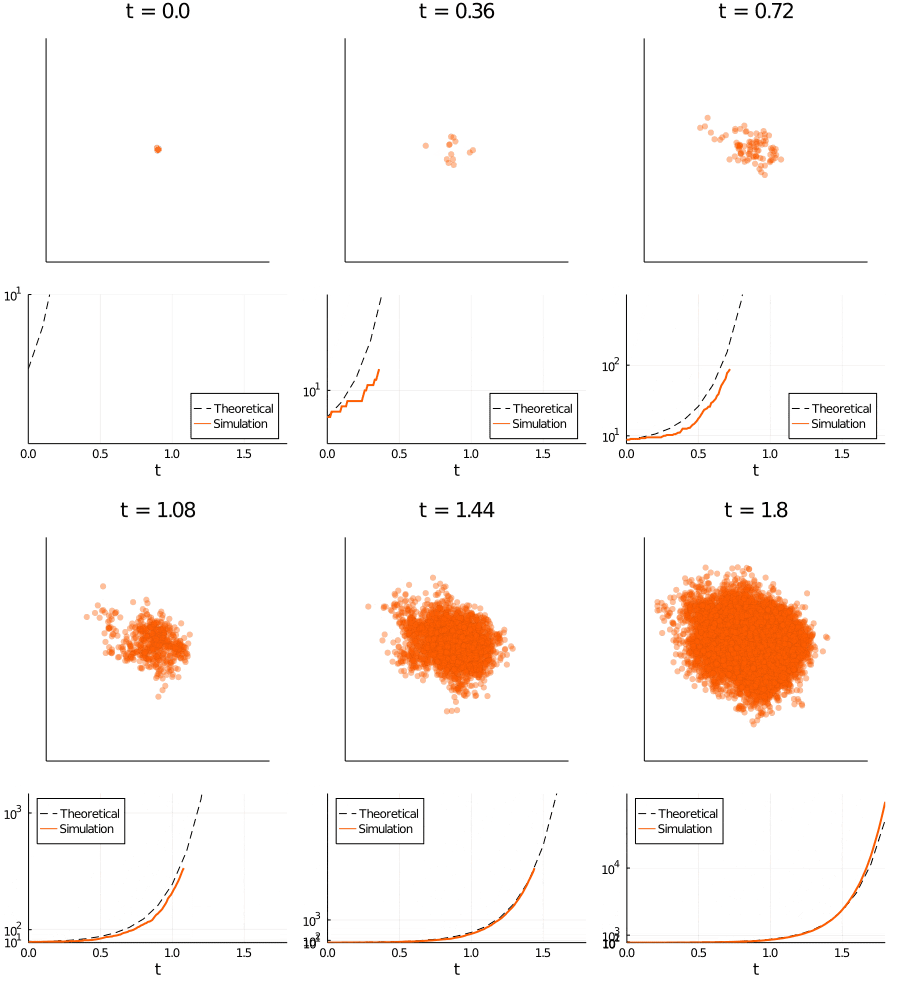
The Case $r>0$
N0 = 50 # 초기 인구수
b = 0.05 # 번식률
d = 0.02 # 사망률
Being a simulation, it may hesitate slightly at first, but because the birth rate is greater than the death rate, explosive growth ultimately occurs.
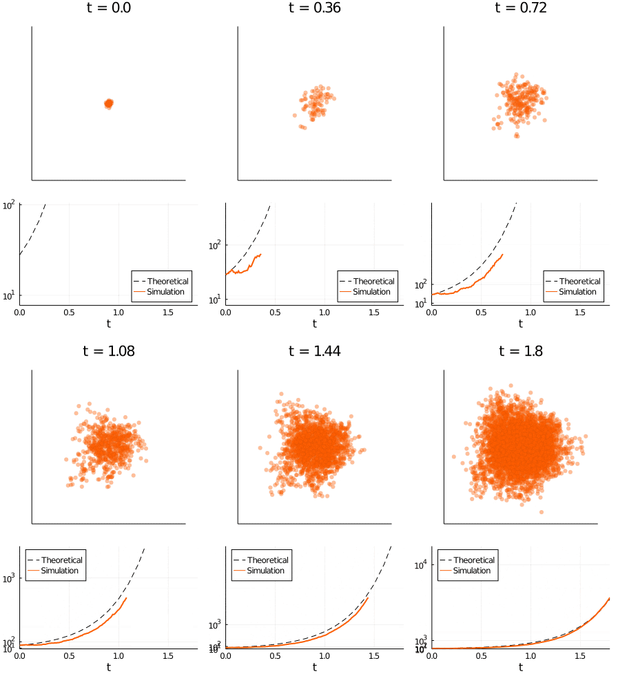
The Case $r<0$
N0 = 50 # 초기 인구수
b = 0.04 # 번식률
d = 0.05 # 사망률
We can see that it follows the theoretical course of extinction almost exactly.
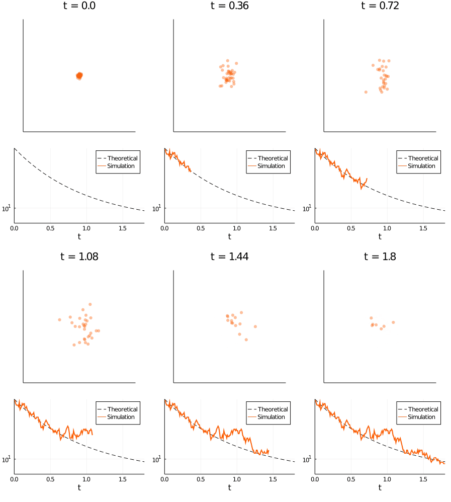
The Case $r=0$
N0 = 50 # 초기 인구수
b = 0.05 # 번식률
d = 0.05 # 사망률
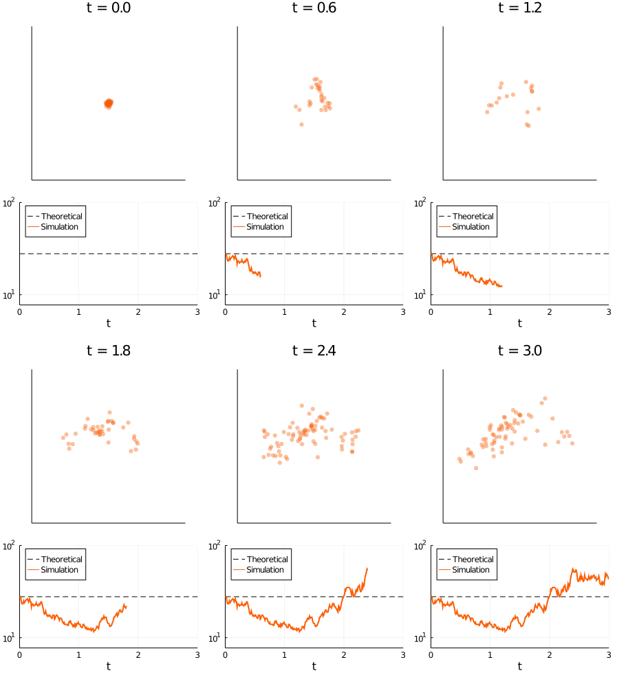
When expressed by a differential equation, the initial value becomes a fixed point so there should be no fluctuation, but in the simulation, due to moment-to-moment luck, it sometimes goes right up to the brink of extinction and then recovers again. This movement can also look like a kind of Brownian motion, and in fact, if you increase the population or lower the birth rate and death rate, it will maintain a somewhat more stable equilibrium state.
- In reality it is geometric Brownian motion.
Code
The following is the Julia code used in this post.
cd(@__DIR__) # 파일 저장 경로

@time using Plots
@time using Random
@time using Distributions
@time using LinearAlgebra
@time using DifferentialEquations

#---

function malthusian_growth!(du,u,p,t)
  N = u[1]
  r = p
  du[1] = dN = r*N
end

u0 = [50.0]
p = 2.65

tspan = (0.,1.8)
prob = ODEProblem(malthusian_growth!,u0,tspan,p)
sol = solve(prob; saveat=(0.0:0.1:1.8))

compare = plot(sol,vars=(0,1),
  linestyle = :dash,  color = :black,
  size = (400,300), label = "Theoretical", legend=:topleft)

#---

N0 = 50 # 초기 인구수
b = 0.05 # 번식률
d = 0.02 # 사망률
max_iteration = 180 # 시뮬레이션 기간
gaussian2 = MvNormal([0.0; 0.0], 0.03I) # 2차원 정규분포

Random.seed!(0)
time_evolution = [] # 인구수를 기록하기 위한
let
  coordinate = rand(gaussian2, N0)'
  N = N0

  anim = @animate for t = (0:max_iteration)/100
    row2 = @layout [a{0.6h}; b]
    figure = plot(size = [300,500], layout = row2)

    plot!(figure[1], coordinate[:,1], coordinate[:,2], Seriestype = :scatter,
      markercolor = RGB(1.,94/255,0.), markeralpha = 0.4, markerstrokewidth	= 0.1,
      aspect_ratio = 1, title = "t = $t",
      xaxis=true,yaxis=true,axis=nothing, legend = false)
      xlims!(figure[1], -10.,10.)
      ylims!(figure[1], -10.,10.)

    replicated = (rand(N) .< b) # 번식 판정
    new_coordinate = coordinate[replicated,:]
    coordinate = coordinate[rand(N) .> d,:] # 사망 판정
    coordinate = cat(coordinate, new_coordinate, dims = 1);

    N = size(coordinate, 1)
    push!(time_evolution, N)
    coordinate = coordinate + rand(gaussian2, N)'

    if t < 0.9
      plot!(figure[2], sol,vars=(0,1),
        linestyle = :dash,  color = :black,
        label = "Theoretical", legend=:bottomright)
    else
      plot!(figure[2], sol,vars=(0,1),
        linestyle = :dash,  color = :black,
        label = "Theoretical", legend=:topleft)
    end
    plot!(figure[2], 0.0:0.01:t, Time_evolution,
      color = RGB(1.,94/255,0.), linewidth = 2, label = "Simulation",
      yscale = :log10, yticks = 10 .^(1:4))
    ylims!(figure[2], 0.,min(time_evolution[end]*2,10000.))
  end
  gif(anim, "malthusian_growth_integration1.gif", fps = 18)
end

#---

function malthusian_growth!(du,u,p,t)
  N = u[1]
  r = p
  du[1] = dN = r*N
end

u0 = [50.0]
p = -1

tspan = (0.,1.8)
prob = ODEProblem(malthusian_growth!,u0,tspan,p)
sol = solve(prob; saveat=(0.0:0.1:1.8))

compare = plot(sol,vars=(0,1),
  linestyle = :dash,  color = :black,
  size = (400,300), label = "Theoretical", legend=:topleft)


#---

N0 = 50 # 초기 인구수
b = 0.04 # 번식률
d = 0.05 # 사망률
max_iteration = 180 # 시뮬레이션 기간
gaussian2 = MvNormal([0.0; 0.0], 0.03I) # 2차원 정규분포

Random.seed!(0)
time_evolution = [] # 인구수를 기록하기 위한
let
  coordinate = rand(gaussian2, N0)'
  N = N0

  anim = @animate for t = (0:max_iteration)/100
    row2 = @layout [a{0.6h}; b]
    figure = plot(size = [300,500], layout = row2)

    plot!(figure[1], coordinate[:,1], coordinate[:,2], Seriestype = :scatter,
      markercolor = RGB(1.,94/255,0.), markeralpha = 0.4, markerstrokewidth	= 0.1,
      aspect_ratio = 1, title = "t = $t",
      xaxis=true,yaxis=true,axis=nothing, legend = false)
      xlims!(figure[1], -10.,10.)
      ylims!(figure[1], -10.,10.)

    replicated = (rand(N) .< b) # 번식 판정
    new_coordinate = coordinate[replicated,:]
    coordinate = coordinate[rand(N) .> d,:] # 사망 판정
    coordinate = cat(coordinate, new_coordinate, dims = 1);

    N = size(coordinate, 1)
    push!(time_evolution, N)
    coordinate = coordinate + rand(gaussian2, N)'


    plot!(figure[2], sol,vars=(0,1),
      linestyle = :dash,  color = :black,
      label = "Theoretical", legend=:topright)
    plot!(figure[2], 0.0:0.01:t, Time_evolution,
      color = RGB(1.,94/255,0.), linewidth = 2, label = "Simulation",
      yscale = :log10, yticks = 10 .^(1:4))
    ylims!(figure[2], 0., 50.)
  end
  gif(anim, "malthusian_growth_integration2.gif", fps = 18)
end


#---

function malthusian_growth!(du,u,p,t)
  N = u[1]
  r = p
  du[1] = dN = r*N
end

u0 = [50.0]
p = 0

tspan = (0.,3.)
prob = ODEProblem(malthusian_growth!,u0,tspan,p)
sol = solve(prob; saveat=(0.0:0.1:3.0))

compare = plot(sol,vars=(0,1),
  linestyle = :dash,  color = :black,
  size = (400,300), label = "Theoretical", legend=:topleft)


#---

N0 = 50 # 초기 인구수
b = 0.05 # 번식률
d = 0.05 # 사망률
max_iteration = 300 # 시뮬레이션 기간
gaussian2 = MvNormal([0.0; 0.0], 0.03I) # 2차원 정규분포

Random.seed!(0)
time_evolution = [] # 인구수를 기록하기 위한
let
  coordinate = rand(gaussian2, N0)'
  N = N0

  anim = @animate for t = (0:max_iteration)/100
    row2 = @layout [a{0.6h}; b]
    figure = plot(size = [300,500], layout = row2)

    plot!(figure[1], coordinate[:,1], coordinate[:,2], Seriestype = :scatter,
      markercolor = RGB(1.,94/255,0.), markeralpha = 0.4, markerstrokewidth	= 0.1,
      aspect_ratio = 1, title = "t = $t",
      xaxis=true,yaxis=true,axis=nothing, legend = false)
      xlims!(figure[1], -10.,10.)
      ylims!(figure[1], -10.,10.)

    replicated = (rand(N) .< b) # 번식 판정
    new_coordinate = coordinate[replicated,:]
    coordinate = coordinate[rand(N) .> d,:] # 사망 판정
    coordinate = cat(coordinate, new_coordinate, dims = 1);

    N = size(coordinate, 1)
    push!(time_evolution, N)
    coordinate = coordinate + rand(gaussian2, N)'


    plot!(figure[2], sol,vars=(0,1),
      linestyle = :dash,  color = :black,
      label = "Theoretical", legend=:topleft)
    plot!(figure[2], 0.0:0.01:t, Time_evolution,
      color = RGB(1.,94/255,0.), linewidth = 2, label = "Simulation",
      yscale = :log10, yticks = 10 .^(1:4))
    ylims!(figure[2], 0., 100.)
  end
  gif(anim, "malthusian_growth_integration3.gif", fps = 18)
end