Classification of Fixed Points in Autonomous Systems
Definition
Given a space $X$ and a function $f \in C^{1}(X,X)$, consider the following vector field given as a differential equation: $$ \dot{x} = f(x) $$ Let $\overline{x}$ be a fixed point of this autonomous system and the eigenvalues of $D f \left( \overline{x} \right)$ be described as $\lambda_{1} , \cdots , \lambda_{m}$.
Hyperbolic: Hyperbolic Fixed Points1
- Hyperbolic: If the real parts of all eigenvalues of $D f \left( \overline{x} \right)$ are not $0$, then $\overline{x}$ is said to be hyperbolic.
$$
\operatorname{Re} \left( \lambda_{1} \right) \ne 0 , \cdots , \operatorname{Re} \left( \lambda_{m} \right) \ne 0
$$
- Saddle: If $\overline{x}$ is hyperbolic and $D f \left( \overline{x} \right)$ has at least one eigenvalue with a positive real part and one with a negative real part, then $\overline{x}$ is called a saddle. $$ \exists i, j \in [1,m] : \operatorname{Re} \left( \lambda_{i} \right) > 0 \land \operatorname{Re} \left( \lambda_{j} \right) < 0 $$
- Sink : If the real parts of all eigenvalues of $D f \left( \overline{x} \right)$ are negative, then $\overline{x}$ is said to be stable and called a sink. $$ \operatorname{Re} \left( \lambda_{1} \right) < 0 , \cdots , \operatorname{Re} \left( \lambda_{m} \right) < 0 $$
- Source : If the real parts of all eigenvalues of $D f \left( \overline{x} \right)$ are positive, then $\overline{x}$ is said to be unstable and called a source. $$ \operatorname{Re} \left( \lambda_{1} \right) > 0 , \cdots , \operatorname{Re} \left( \lambda_{m} \right) > 0 $$
Elliptic: Elliptic Fixed Points2
- Elliptic, Center : If all eigenvalues of $D f \left( \overline{x} \right)$ are purely imaginary, then $\overline{x}$ is said to be elliptic and called a center. $$ \operatorname{Im} \left( \lambda_{1} \right) = \lambda_{1} , \cdots , \operatorname{Im} \left( \lambda_{m} \right) = \lambda_{m} $$
- $\re$ and $\im$ are functions that extract only the real and imaginary parts, respectively, from complex numbers.
Description
Although not explicitly stated in the definition, the distinction between hyperbolic and non-hyperbolic can be roughly equated with the simplicity of the system. In analyzing systems dynamically, the primary issue often arises when an eigenvalue is $0$; being hyperbolic means one does not have to worry about such nuisances, simplifying the analysis.
Examples
Consider the Duffing oscillator as an example: $$ \begin{align*} \dot{x} =& y \\ \dot{y} =& x - x^{3} - \delta y \qquad , \delta \ge 0 \end{align*} $$ The fixed points of the Duffing oscillator are $(x,y) = (0,0) , (\pm 1 , 0)$ and its Jacobian is: $$ D \mathbf{f} = \begin{bmatrix} 0 & 1 \\ 1 - 3 x^{2} & - \delta \end{bmatrix} $$ Thus, the Jacobian at the fixed points is: $$ D \mathbf{f} (0,0) = \begin{bmatrix} 0 & 1 \\ 1 & - \delta \end{bmatrix} \\ D \mathbf{f} (\pm1,0) = \begin{bmatrix} 0 & 1 \\ -2 & - \delta \end{bmatrix} $$ Calculating the eigenvalues yields, when $(0,0)$: $$ \det ( D \mathbf{f} (0,0) - \lambda E ) = \det \begin{bmatrix} -\lambda & 1 \\ 1 & -\lambda - \delta \end{bmatrix} = \lambda^{2} + \delta \lambda - 1 $$ According to the quadratic formula: $$ \lambda_{1,2} = {{ -\delta \pm \sqrt{\delta^{2} + 4 } } \over { 2 }} $$ The eigenvalues of $D \mathbf{f} (0,0)$ always include a positive and a negative number, thus the fixed point $(0,0)$ is a saddle. Similarly, calculating the eigenvalues for $D \mathbf{f} (\pm1,0)$ yields: $$ \lambda_{1,2} = {{ -\delta \pm \sqrt{\delta^{2} - 8 } } \over { 2 }} $$ Therefore, the eigenvalues of $D \mathbf{f} (\pm1,0)$ are all negative when $\delta > 0$, and the fixed point $(\pm1,0)$ is a sink. However, when $\delta = 0$, the eigenvalues are purely imaginary $\lambda_{1,2} = \pm \sqrt{2} i$, making the fixed point $(\pm1,0)$ a center.
In the above example, we determined the Jacobian at each fixed point and examined how stability changes based on the settings of the parameter $\delta$. Such analysis, if the system is represented by a vector field, is a common approach used in any paper on dynamics. At least once, be sure to try it yourself.
