📂Functions

Dirac Delta Function

Definition

A function satisfying the following two conditions is called the Dirac delta function.

$$ \delta (x) = \begin{cases} 0, & x\neq 0 \\ \infty , & x=0 \end{cases} $$

$$ \int_{-\infty}^{\infty}{\delta (x) dx}=1 $$

Explanation¹

Since $\delta(x)$ diverges at $x=0$, it is not actually a function. Although it can be described rigorously in a mathematical sense, this is not easy to understand for undergraduates across many majors who will use this function extensively in their calculations. Because the strange definition of the delta function does not cause much trouble in computations, it is fine to just learn how to use it without understanding the precise definition. This is much like how $\dfrac{dy}{dx}$ is not actually a fraction, yet treating it as one and manipulating the numerator and denominator separately still yields correct results such as the chain rule. However, since there is a point where it diverges, keep in mind that when computing, $\delta$ is never used on its own; its value can only be determined when it is always inside an integral.

The Kronecker delta $\delta_{ij}$ takes the value $1$ only when the indices are equal, much like a discrete version of the Dirac delta function. In other words, the Dirac delta function is a continuous version of the Kronecker delta.

$$ \delta_{ij} = \begin{cases} 1, & i = j \\ 0, & i \ne j \end{cases} $$

Geometric Meaning

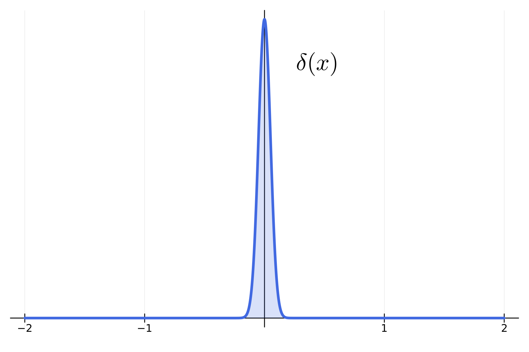
As in the figure above, the delta function is drawn as a spike that rises infinitely narrow and tall at the origin while the area under the graph is $1$. This intuition can be made concrete as the limit of a sequence of functions consisting of ordinary functions. Consider a rectangular function $R_{n}$ of height $n$ and width $\dfrac{1}{n}$, and an isosceles triangular function $T_{n}$ of height $n$ and base $\dfrac{2}{n}$.

$$ R_{n}(x) = \begin{cases} n, & |x| \le \dfrac{1}{2n} \\ 0, & \text{otherwise} \end{cases} \qquad T_{n}(x) = \begin{cases} n - n^{2} |x|, & |x| \le \dfrac{1}{n} \\ 0, & \text{otherwise} \end{cases} $$

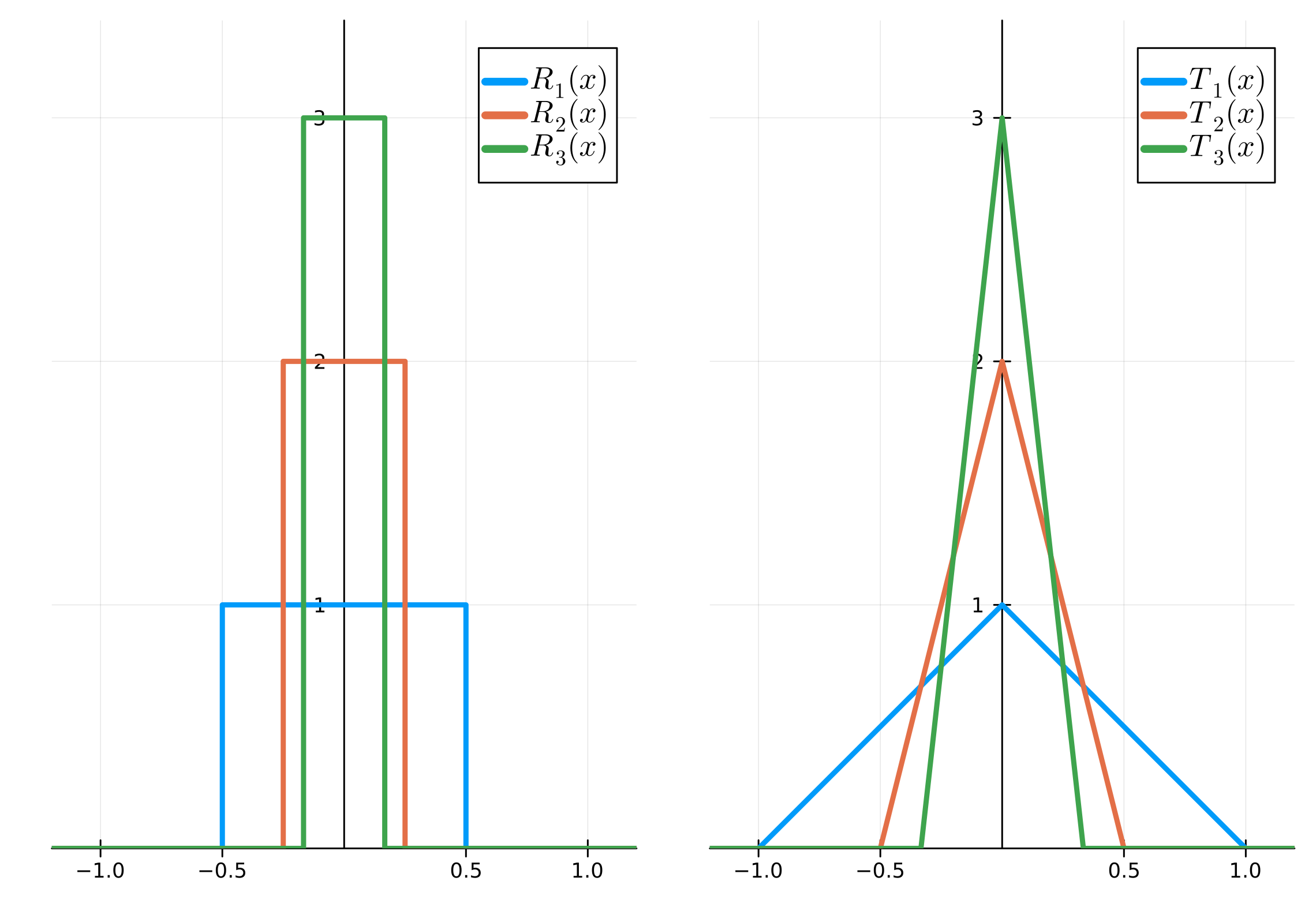
As $n$ grows larger, both functions become progressively narrower and taller, yet the area under the graph remains constant at $1$ for every $n$.

$$ \int_{-\infty}^{\infty} R_{n}(x) dx = n \cdot \frac{1}{n} = 1 \qquad \int_{-\infty}^{\infty} T_{n}(x) dx = \frac{1}{2} \cdot \frac{2}{n} \cdot n = 1 $$

Therefore, in the limit $n \to \infty$, the function value becomes $0$ everywhere except at $x = 0$, and yet the total integral still remains $1$. The delta function is precisely the object that can be imagined through this limit.

$$ \delta (x) = \lim_{n \to \infty} R_{n}(x) = \lim_{n \to \infty} T_{n}(x) $$

Properties

Let $f$ be an ordinary function that is not a delta function. Since $\delta (x)$ is $0$ everywhere except at $x = 0$, in the product $f(x) \delta (x)$ only the single value $f(0)$ of $f$ survives.

(a) sampling property: Integrating the product with the delta function extracts the value of $f$ at a single point.

$$ f(x) \delta (x) = f(0) \delta (x) \implies \int_{-\infty}^{\infty} f(x) \delta (x) dx = f(0) \int_{-\infty}^{\infty} \delta (x) dx = f(0) $$

(b) Translation: The sampling property holds just as well for $\delta (x - a)$, which shifts the spike to $x = a$.

$$ \delta (x - a) = \begin{cases} 0, & x \neq a \\ \infty, & x = a \end{cases} \qquad \int_{-\infty}^{\infty} \delta (x - a) dx = 1 $$

$$ f(x) \delta (x - a) = f(a) \delta (x - a) \implies \int_{-\infty}^{\infty} f(x) \delta (x - a) dx = f(a) $$

(c) Even Function, Scaling: The delta function is an even function, and for a scaling by a constant $a \neq 0$ the following holds.

$$ \delta (-x) = \delta (x) \qquad \delta (ax) = \frac{1}{|a|} \delta (x) $$

(d) Three-Dimensional Delta Function: For the position vector $\mathbf{r} = (x, y, z)$, it is defined as the product of the delta functions of each component, and its integral over the volume element $d\tau = dx dy dz$ is $1$.

$$ \delta^{3} (\mathbf{r}) = \delta (x) \delta (y) \delta (z) \qquad \int \delta^{3} (\mathbf{r}) d\tau = 1 $$

The sampling property also holds in three dimensions as it is.

$$ \int f( \mathbf{r} ) \delta^{3} (\mathbf{r} - \mathbf{a}) d\tau = f(\mathbf{a}) $$

Applications

The fundamental forces of nature, including gravity and electric force, follow the inverse-square law, in which the magnitude is inversely proportional to the square of the distance. That is, when the source is at the origin, the field they create is proportional to the vector function $\dfrac{\hat{\mathbf{r}}}{r^{2}}$. Since this vector function has a shape spreading out in all directions from the origin, its divergence looks as though it would be large, but when one actually computes it, the result is $0$. In spherical coordinates, the divergence of a vector function having only a radial component $v_{r}$ is $\nabla \cdot \mathbf{v} = \dfrac{1}{r^{2}} \dfrac{\partial}{\partial r} \left( r^{2} v_{r} \right)$, so it is as follows.

$$ \nabla \cdot \dfrac{\hat{\mathbf{r}}}{r^{2}} = \dfrac{1}{r^{2}} \frac{\partial}{\partial r} \left( r^{2} \cdot \dfrac{1}{r^{2}} \right) = \dfrac{1}{r^{2}} \frac{\partial}{\partial r} (1) = 0 $$

Of course, since $\dfrac{\hat{\mathbf{r}}}{r^{2}}$ is not defined at $r = 0$, to be precise $\nabla \cdot \dfrac{\hat{\mathbf{r}}}{r^{2}}$ is a function that is $0$ everywhere with $r \ne 0$. On the other hand, if we integrate this divergence over the volume of a sphere $\mathcal{V}$ centered at the origin with radius $R$, the story changes. By the divergence theorem, the volume integral turns into a surface integral over the surface $\mathcal{S}$ of the sphere, and on the surface $r = R$ is fixed, so the infinitesimal area vector is $d\mathbf{a} = R^{2} \sin\theta d\theta d\phi \hat{\mathbf{r}}$, giving the following.

$$ \int_{\mathcal{V}} \nabla \cdot \dfrac{\hat{\mathbf{r}}}{r^{2}} dV = \oint_{\mathcal{S}} \dfrac{\hat{\mathbf{r}}}{R^{2}} \cdot d\mathbf{a} = \oint_{\mathcal{S}} \dfrac{\hat{\mathbf{r}}}{R^{2}} \cdot \left( R^{2} \sin\theta d\theta d\phi \hat{\mathbf{r}} \right) = \int_{0}^{\pi} \sin\theta d\theta \int_{0}^{2\pi} d\phi = 4\pi $$

This value is independent of the radius $R$ of the sphere. No matter how small we shrink the sphere, the integral is still $4\pi$, and the integral over all of space with the radius grown without bound is likewise $4\pi$. In the end, $\nabla \cdot \dfrac{\hat{\mathbf{r}}}{r^{2}}$ is $0$ everywhere except the origin, yet integrating it yields a nonzero constant value, and this is exactly the property of the delta function. The entire divergence is concentrated at the single point of the origin, and it can be expressed using the three-dimensional delta function as follows.

$$ \nabla \cdot \dfrac{\hat{\mathbf{r}}}{r^{2}} = 4\pi \delta^{3}(\mathbf{r}) $$

Using this, even the integral below, which looks complicated at first glance, can be computed easily. When $\mathcal{V}$ is a region containing the origin, by the property of the delta function only the value at the origin, $0^{2} + 2$, survives in place of $r^{2} + 2$.

$$ \begin{align*} \int_{\mathcal{V}} (r^{2} + 2) \nabla \cdot \dfrac{\hat{\mathbf{r}}}{r^{2}} dV &= \int_{\mathcal{V}} (r^{2} + 2) 4\pi \delta^{3}(\mathbf{r}) dV \\ &= 4\pi (0^{2} + 2) \int_{\mathcal{V}} \delta^{3}(\mathbf{r}) dV \\ &= 8\pi \end{align*} $$