Nullclines in Mathematical Analysis
Definition
Isocline
Given a set of curves, the set of points with the same slope is called an isocline.
Nullcline
Given an $p$-dimensional ordinary differential equation as in $\dot{\mathbf{x}} = \mathbf{f} \left( \mathbf{x} \right)$, the isocline with the slope $0$ for the $k$ coordinate $x_{k}$ is called a nullcline. More specifically, the $N_{k}$ nullcline for the $k$ coordinate can be defined as follows: $$ N_{k} := \left\{ \mathbf{x} = \left( x_{1} , \cdots , x_{p} \right) \in \mathbb{R}^{p} : {\frac{ d x_{k} }{ d t }} = 0 \right\} $$
Explanation

Nullclines are a useful tool for analyzing dynamical systems, especially when visualized in a two-dimensional plane1. While nullclines alone cannot capture all details of the system, they provide a rough overview of the system’s behavior, and the intersections of all nullclines represent the set of fixed points. $$ \bigcap_{k=1}^{p} N_{k} = \left\{ \mathbf{x}_{0} : \mathbf{f} \left( \mathbf{x}_{0} \right) = \mathbf{0} \right\} $$
Practice
$$ \begin{align*} \dot{x} =& x + y \\ \dot{y} =& \mu y + x^{2} - xy \end{align*} $$
The following visualizes the nullclines for the given ordinary differential equations when $\mu = - 1.755$. As mentioned earlier, observing the nullclines allows us to approximate the locations of two fixed points, and in particular, $(x,y) = (0,0)$ can be easily verified as a trivial fixed point.

The specific process is as follows:
- Numerically, we assume that it is impossible to find points where exactly $\dot{x} = 0$ or $\dot{y} = 0$. The plane is divided into a sufficiently large number of grids, and the vector $\left( \dot{x} , \dot{y} \right) = \mathbf{f} (x,y)$ is calculated at all these points.
- Divide the regions into positive and negative for each of $\dot{x}$ and $\dot{y}$. The result will probably be two matrices consisting of true and false values.
- According to the Intermediate value theorem, there exist points satisfying $\dot{x} = 0$ or $\dot{y} = 0$ where the positive and negative regions meet. Find these boundary points by taking the difference of the matrices consisting of true and false values. Perform this operation in both the row and column directions. Note that when taking the difference of the matrix, the size changes, so appropriate padding should be applied.
Complete Code
The following is the Julia code to reproduce the nullclines shown in this post.
using Plots, LinearAlgebra
μ = -1.755
h = 0.1

f(v) = [v[1] + v[2], μ*v[2] + v[1]^2 - v[1]*v[2]]

pos = collect(Base.product(-1.5:0.001:.5, -.5:0.001:2))
dir = f.(pos)
x_ = first.(dir)
y_ = last.(dir)
null_x = .!iszero.([diff(x_ .> 0, dims = 1); zeros(Int64, 1, size(x_, 2))] +
[diff(x_ .> 0, dims = 2) zeros(Int64, size(x_, 1), 1)])
null_y = .!iszero.([diff(y_ .> 0, dims = 1); zeros(Int64, 1, size(y_, 2))] +
[diff(y_ .> 0, dims = 2) zeros(Int64, size(y_, 1), 1)])
plot(xlims = [-1.5,.5], ylims = [-.5,2], xlabel = "x", ylabel = "y", size = [600, 600])
scatter!(first.(pos[null_x]), last.(pos[null_x]), label = "dx/dt = 0", color =  :red, msw = 0, alpha = .5, ms = 0.5)
scatter!(first.(pos[null_y]), last.(pos[null_y]), label = "dy/dt = 0", color = :blue, msw = 0, alpha = .5, ms = 0.5)
png("null_clines.png")
Strogatz. (2015). Nonlinear Dynamics And Chaos: With Applications To Physics, Biology, Chemistry, And Engineering(2nd Edition): p148. ↩︎
