📂Statistical Analysis

Model Diagnostics in Regression Analysis

Necessity

In the case of simple regression analysis, considering the independent and dependent variables only amounts to $2$ dimensions, so one can tell at a glance whether the analysis was done properly. However, in the case of multiple regression analysis, once it goes beyond $3$ dimensions it becomes difficult to draw as a picture, so it is hard to verify whether the analysis really fits well. There are cases where the assumptions of regression analysis are not properly satisfied yet the hypothesis test is passed, and in that case the analysis is simply wrong.

An analysis goes wrong mainly when (1) the data does not fit the linear model, or (2) there is a severe gap between the analysis results and the actual understanding of the data. Model diagnostics are carried out to check whether or not the data fits the linear model.

Diagnostics¹

Saying that the data does not fit the linear model simply means that the data does not lie in the shape of a straight line. Whether the data fits the linear model or not is judged by looking at the standardized residual plot and performing model diagnostics. This kind of residual analysis is quite an ingenious method, devised because it is difficult to draw a straight line in high dimensions. It is fair to say that this is the very reason residuals are calculated in the first place.

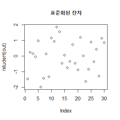If the following four conditions are satisfied in the residual plot, the model diagnostics are considered to have passed.

• (i) Linearity: The residuals should be distributed symmetrically around $0$.
  • This is an assumption that is one and the same as the essence of regression analysis; since the goal of regression analysis is to obtain a straight line, there is no point if linearity is not satisfied. Of course, the very reason for using regression analysis in the first place is that one suspects linearity exists, so in actual analyses it tends to be satisfied very easily.
• (ii) Homoscedasticity: The residuals should be evenly distributed.
  • If the variability suddenly becomes small in a particular interval, it is hard to regard the data as having been obtained through the same process. For instance, one cannot help but consider whether there were problems such as differences among the surveyors collecting the statistics, or mistakes. If there is a problem such as the variance growing or shrinking as the data goes on, it can be partially resolved by transforming the variables.
• (iii) Independence: There should be no pattern among the residuals.
  • The residuals having some pattern violates the assumption of regression analysis that the error is completely random. Conversely, a lack of independence means there may be a rule we do not yet know, such as autocorrelation. In this case, rather than trying to work around it, it is better to find a more suitable tool such as time series analysis. If it is severe, it stands out enough to be noticed at a glance; if it is not that bad, it may be regarded as no big problem. One word of caution: do not carelessly reach for the Durbin-Watson test to check independence. Strictly speaking, the Durbin-Watson test detects autocorrelation among residuals separated by a fixed interval; it does not establish independence. If there is an obvious pattern even at a glance, one must not believe in independence just because the Durbin-Watson test was passed.
• (iv) Normality: The residuals should look as if they follow the standard normal distribution.
  • Unlike the other assumptions, normality allows for objective diagnosis, such as the Shapiro-Wilk test or the Jarque-Bera test. Nevertheless, the problem is not so simple, since what mainly deals a serious blow to normality is outliers. In such cases, if the analyst can personally look at the data corresponding to the outliers and directly explain the phenomenon, it is not a big problem. One word of caution: do not blindly remove data just because they are outliers. For example, if there are $300$ samples and about $3$ outliers lying beyond six sigma ($\pm 3 \sigma$) above and below, that is normal. Having too many outliers is a problem, but unlike in probability distribution theory, having excessively few outliers does not mean the data properly follows the normal distribution either.

The above four conditions are arranged not arbitrarily but in order of importance, and this hierarchy can be understood not only through intuition or experience but also by looking at the theoretical derivation of the hypothesis test for regression coefficients². When engaging in actual statistical analysis, not all data turns out neatly, so there are times when one has to compromise on some conditions. In such cases, normality can be given up to some extent even if there are somewhat problematic aspects, such as many outliers or a slight skew.

Such model diagnostics rely to a large extent on eyeballing, and an understanding of the data is essential. Finding what is wrong is the first problem; how to fix what is wrong is the second problem. The best way to develop this ability is to see as many cases as possible while engaging in actual analyses.

Code

Below is the R code that outputs the residual plot.

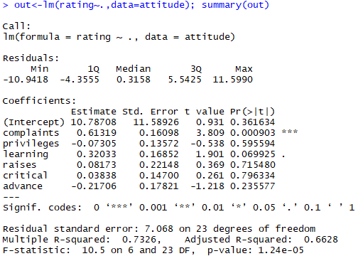
out<-lm(rating~.,data=attitude); summary(out)
win.graph(5,5); plot(rstudent(out),main="표준화된 잔차")