📂Dynamical Systems

Food Chain System in Dynamics

Model ¹

$$ \begin{align*} \dot{R} =& R \left( 1 - {\frac{ R }{ K }} \right) - {\frac{ x_{c} y_{c} C R }{ R + R_{0} }} \\ \dot{C} =& x_{c} C \left( {\frac{ y_{c} R }{ R + R_{0} }} - 1 \right) - {\frac{ x_{p} y_{p} P C }{ C + C_{0} }} \\ \dot{P} =& x_{p} P \left( {\frac{ y_{p} C }{ C + C_{0} }} - 1 \right) \end{align*} $$

Variables

• $R(t)$: Density of the resource at time $t$.
• $C(t)$: Density of the consumer at time $t$.
• $P(t)$: Density of the predator at time $t$.

Parameters

• $K = 0.94$: The carrying capacity of the resource.
• $x_{c} = 0.4$, $y_{c} = 1.7$, $R_{0} = 0.16129$: Parameters related to the consumer’s predation on the resource.
• $y_{p} = 5.0$, $x_{p} = 0.08$, $C_{0} = 0.5$: Parameters related to the predator’s predation on the consumer.

Description

The introduced $3$-dimensional food-chain system has the resource following the logistic growth model and can be seen as two coupled Lotka–Volterra predator–prey models — resource–consumer and consumer–predator — i.e., a coupled dynamical system.

A system composed by combining such simple subsystems would not normally be complicated, but by incorporating a Holling type II response function between $R-C-P$ the system becomes chaotic. Indeed, the bifurcation diagram obtained by varying $K, y_{c}, y_{p}$ is as follows.

From a research perspective, being familiar with such systems can add value to a paper. Similarly, the Lorenz attractor is a $3$-dimensional chaotic system, but it is so famous and widely used that it is not attractive as a benchmark; moreover, it can now be represented by polynomial functions of degree at most $2$, which may make its complexity seem reduced. By contrast, the food-chain system already carries an intuitive ecological interpretation, is chaotic, and its equations include rational functions, making it relatively more complex².

Transient chaos ^{3 4}

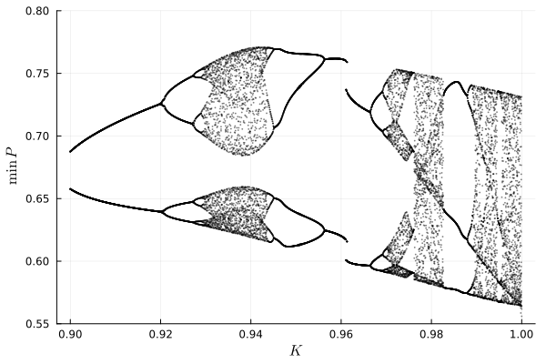
Meanwhile, for parameter values $x_{c} = 0.4$, $y_{c} = 2.009$, $x_{p} = 0.08$, $y_{p} = 2.876$, $R_{0} = 0.16129$, and $C_{0} = 0.5$, in the vicinity of $K \approx 0.99976$ one observes transient chaos. When drawing this bifurcation diagram, note that transient chaos requires repeated simulations across many initial conditions.

The following plot shows that, when $K = 0.99976 + 2\times 10^{-4}$, the distribution of transient lifetimes over varying initial conditions follows an exponential distribution.

Below is Julia code to reproduce this.

function RK4(f::Function, v::AbstractVector, h=1e-2)
    V1 = f(v)
    V2 = f(v + (h/2)*V1)
    V3 = f(v + (h/2)*V2)
    V4 = f(v + h*V3)
    return v + (h/6)*(V1 + 2V2 + 2V3 + V4), V1
end

function factory_foodchain2(K::Number; ic = [0., 0.4rand() + 0.6, 0.4rand() + 0.15, 0.5rand() + 0.3], tspan = 0:1e-2:10)
     xc,    yc,   xp,    yp,      R0,  C0 = (
    0.4, 2.009, 0.08, 2.876, 0.16129, 0.5)
    function sys(v::AbstractVector)
        _,R,C,P = v

        dt = 1
        dR = R*(1 - frac(R,K)) - xc*yc*frac(C*R, R + R0)
        dC = xc*C*(frac(yc*R, R + R0) - 1) - xp*yp*frac(P*C, C + C0)
        dP = xp*P*(frac(yp*C, C + C0) - 1)
        return [dt, dR, dC, dP]
    end

    len_t_ = length(tspan); h = tspan.step.hi
    v = ic; DIM = length(v)
    traj = zeros(2+len_t_, 2DIM); traj[1, 1:DIM] = v

    tk = 0
    while tk ≤ len_t_
        t,_,_,_ = v
        v, dv = RK4(sys, v, h)

        if t ≥ first(tspan)
            tk += 1
            traj[tk+1,         1:DIM ] =  v
            traj[tk  , DIM .+ (1:DIM)] = dv
        end
    end
    return traj[1:(end-2), :]
end
factory_foodchain2(T::Type, args...; kargs...) =
DataFrame(factory_foodchain2(args...; kargs...), ["t", "R", "C", "P", "dt", "dR", "dC", "dP"])[:, Not(:dt)]

hrzn = []
vrtl = []
@time for k in 0.9:0.0001:1
    for _ in 1:500
        traj = factory_foodchain2(DataFrame, k, tspan = 0:1e-1:5000)[40000:end,:]
        bits = arglmin(traj.P)
        if maximum(traj.P) > 0.55
            push!(hrzn, fill(k, length(bits)))
            push!(vrtl, traj.P[bits])
            break
        else
            println("k: $k should be tried again")
        end            
    end
end
using LaTeXStrings
scatter([hrzn...;], [vrtl...;], ylims = [0.55, 0.8], yticks = 0.55:0.05:0.8, xticks = 0.9:0.02:1,
    ms = 1, msw = 0, color = :black, alpha = 0.5, legend = :none, xlabel = L"K", ylabel = L"\min P")
png("bifurcaiton.png")

tau_ = zeros(Int64, 100000)
@showprogress @threads for k in eachindex(tau_)
    traj = factory_foodchain2(DataFrame, 0.99976 + 2e-4, ic = rand(4), tspan = 0:1e-0:5000)
    tau = findlast(diff(cumsum(traj.P .< 0.55)) .== 0)
    tau_[k] = !isnothing(tau) ? tau : -1
end
freq = [count(x .≤ tau_ .< x + 250) for x in 250:250:4750]
scatter(250:250:4750, freq ./ sum(freq), yscale = :log10, xticks = 0:1000:5000, xlims = [0, 5000], yticks = [1e-1, 1e-2], color = :white, legend = :none, xlabel = "transient lifetime", ylabel = "frequency")