📂Dynamical Systems

Hastings-Powell System

Model ¹

$$ \begin{align*} \frac{dX}{dT} =& R_{0} X \left( 1 - \frac{X}{K_{0}} \right) - C_{1} \frac{A_{1} X}{B_{1} + X} Y \\ \frac{dY}{dT} =& \frac{A_{1} X}{B_{1} + X} Y - \frac{A_{2} Y}{B_{2} + Y} Z - D_{1} Y \\ \frac{dZ}{dT} =& C_{2} \frac{A_{2} Y}{B_{2} + Y} Z - D_{2} Z \end{align*} $$

Variables

• $X(T)$: The population size of species $Y$ that is preyed upon at time $T$.
• $Y(T)$: At time $T$, the population size of the species that consumes $X$ and is consumed by $Z$.
• $Z(T)$: At time $T$, the population size of the species that consumes $Y$.

Parameters

• $R_{0}$: The intrinsic growth rate of $X$.
• $K_{0}$: The carrying capacity of $X$.
• $C_{1}^{-1}, C_{2}$: The conversion rates for $Y$ and $Z$, respectively.
• $A_{1}, A_{2}, B_{1}, B_{2}$: Coefficients related to saturation according to the Holling type II functional response.

Explanation

Food chain system: $$ \begin{align*} \dot{R} =& R \left( 1 - {\frac{ R }{ K }} \right) - {\frac{ x_{c} y_{c} C R }{ R + R_{0} }} \\ \dot{C} =& x_{c} C \left( {\frac{ y_{c} R }{ R + R_{0} }} - 1 \right) - {\frac{ x_{p} y_{p} P C }{ C + C_{0} }} \\ \dot{P} =& x_{p} P \left( {\frac{ y_{p} C }{ C + C_{0} }} - 1 \right) \end{align*} $$

The sole reason this post was written is to point out that there is no essential difference between the food chain system and the Hastings–Powell system. Some papers distinguish the two, while others treat them as the same without explicit notation; if one were to argue, it is closer to the latter.

Of course, the equations are not exactly identical — some parameters have different degrees of freedom — but in both cases the models are ecosystem models that assume the presence of a specialized predator.

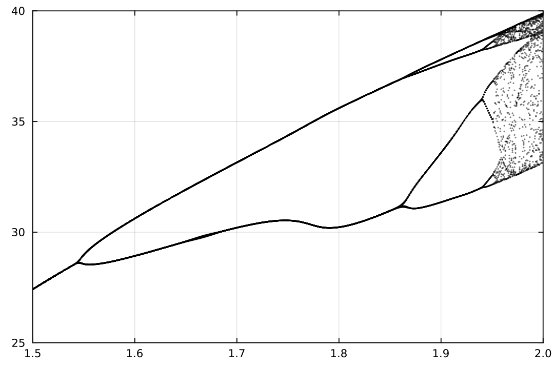
$$ \begin{align*} \dot{v_{1}} =& a_{0} v_{1} - b_{0} v_{1}^2 - \frac{w_{0} v_{1} v_{2}}{d_{0} + v_{1}} \\ \dot{v_{2}} =& \frac{w_{1} v_{1} v_{2}}{d_{1} + v_{1}} - \frac{w_{2} v_{2} v_{3}}{d_{2} + v_{2}} - a_{1} v_{2} \\ \dot{v_{3}} =& \frac{w_{3} v_{2} v_{3}}{d_{3} + v_{2}} - c_{3} v_{3} \end{align*} $$ The following is expressed as $X = v_{1}$, $Y = v_{2}$, $Z = v_{3}$, with coefficients set to $b_{0} = 0.05$, $w_{0} = 1$, $d_{0} = 10$, $w_{1} = 2$, $d_{1} = 10$, $w_{2} = 1.5$, $d_{2} = 10$, $a_{1} = 1$, $w_{3} = 2$, $d_{3} = 20$, $c_{3} = 0.7$, and with $a_{0} \in [1.5, 2.0]$ chosen as the bifurcation parameter; the bifurcation diagram was produced².

Code

The following is Julia code that reproduces the above bifurcation diagram.

function RK4(f::Function, v::AbstractVector, h=1e-2)
    V1 = f(v)
    V2 = f(v + (h/2)*V1)
    V3 = f(v + (h/2)*V2)
    V4 = f(v + h*V3)
    return v + (h/6)*(V1 + 2V2 + 2V3 + V4), V1
end

function arglmax(x)
    bits = circshift(x, 1) .< x .> circshift(x, -1)
    bits[1] = false
    bits[end] = false
    return findall(bits)
end

frac(x, y) = x ./ y
function factory_hastingpowell(a0::Number; ic = [0., 1, 1, 1], tspan = 0:1e-2:10)
      b0, w0, d0, w1, d1,  w2, d2, a1, w3, d3,  c3 = (
    0.05,  1, 10,  2, 10, 1.5, 10,  1,  2, 20, 0.7 )
    function sys(v::AbstractVector)
        _,v1,v2,v3 = v

        dt = 1
        dv1 = a0*v1 - b0*v1^2 - w0*frac(v1*v2, d0 + v1)
        dv2 = w1*frac(v1*v2, d1 + v1) - w2*frac(v2*v3, d2 + v2) - a1*v2
        dv3 = w3*frac(v2*v3, d3 + v2) - c3*v3
        return [dt, dv1, dv2, dv3]
    end
        
    len_t_ = length(tspan); h = tspan.step.hi
    v = ic; DIM = length(v)
    traj = zeros(2+len_t_, 2DIM); traj[1, 1:DIM] = v

    tk = 0
    while tk ≤ len_t_
        t,_,_,_ = v
        v, dv = RK4(sys, v, h)

        if t ≥ first(tspan)
            tk += 1
            traj[tk+1,         1:DIM ] =  v
            traj[tk  , DIM .+ (1:DIM)] = dv
        end
    end
    return traj[1:(end-2), :]
end
factory_hastingpowell(T::Type, args...; kargs...) =
DataFrame(factory_hastingpowell(args...; kargs...), ["t", "v1", "v2", "v3", "dt", "dv1", "dv2", "dv3"])[:, Not(:dt)]

hrzn = []
vrcl = []
for a0 = 0.15:0.001:2.0
    data = factory_hastingpowell(DataFrame, a0, tspan = 0:1e-2:1000)[50001:end, :]
    bits = arglmax(data.v1)
    push!(hrzn, [a0 for _ in bits])
    push!(vrcl, data.v1[bits])
end
scatter([hrzn...;], [vrcl...;], ms = 1, msw = 0, color = :black, alpha = 0.5, legend = :none, xlims = [1.5, 2.0], ylims = [25, 40])