Vanishing Gradient

Introduction¹ ² ³

Consider an artificial neural network formed by repeatedly composing weights $\mathbf{W}^{(1)}, \dots, \mathbf{W}^{(N)}$ and an activation function $\sigma$. For an input $\mathbf{h}^{(0)} = \mathbf{x}$, let the value of each layer be as follows.

$$ \mathbf{h}^{(\ell)} = \overline{\sigma}\left( \mathbf{z}^{(\ell)} \right), \qquad \mathbf{z}^{(\ell)} = \mathbf{W}^{(\ell)} \mathbf{h}^{(\ell-1)} + \mathbf{b}^{(\ell)} \qquad (\ell = 1, \dots, N) $$

Here $\overline{\sigma}$ is the activation function applied componentwise. Suppose the loss function $\mathcal{L}$ is a function of the network’s output $\mathbf{h}^{(N)}$. To train the network with gradient descent, we need the gradient of $\mathcal{L}$ with respect to the weights of each layer. By the chain rule, the gradient with respect to the weights of the $\ell$-th layer is as follows.

$$ \frac{\partial \mathcal{L}}{\partial \mathbf{W}^{(\ell)}} = \frac{\partial \mathcal{L}}{\partial \mathbf{h}^{(\ell)}} \cdot \frac{\partial \mathbf{h}^{(\ell)}}{\partial \mathbf{z}^{(\ell)}} \cdot \frac{\partial \mathbf{z}^{(\ell)}}{\partial \mathbf{W}^{(\ell)}} \tag{1} $$

Here $\partial \mathbf{z}^{(\ell)}/\partial \mathbf{W}^{(\ell)}$ depends only on the input $\mathbf{h}^{(\ell-1)}$ entering that layer, so it does not shrink as the network gets deeper. In contrast, $\partial \mathcal{L}/\partial \mathbf{h}^{(\ell)}$ is the term in which the Jacobian matrices of the later layers are multiplied repeatedly.

$$ \frac{\partial \mathcal{L}}{\partial \mathbf{h}^{(\ell)}} = \frac{\partial \mathcal{L}}{\partial \mathbf{h}^{(N)}} \cdot \frac{\partial \mathbf{h}^{(N)}}{\partial \mathbf{h}^{(N-1)}} \cdot \frac{\partial \mathbf{h}^{(N-1)}}{\partial \mathbf{h}^{(N-2)}} \cdots \frac{\partial \mathbf{h}^{(\ell+1)}}{\partial \mathbf{h}^{(\ell)}} = \frac{\partial \mathcal{L}}{\partial \mathbf{h}^{(N)}} \prod_{k=\ell+1}^{N} \frac{\partial \mathbf{h}^{(k)}}{\partial \mathbf{h}^{(k-1)}} $$

That is, if we denote the Jacobian matrix between two adjacent layers by $J^{(k)} := \partial \mathbf{h}^{(k)} / \partial \mathbf{h}^{(k-1)}$, it can be written as below, and since $\left\| AB \right\| \le \left\| A \right\| \left\| B \right\|$ holds for matrix norms, its magnitude is bounded above by the product of the norms of the Jacobian matrices, as follows.

$$ \frac{\partial \mathcal{L}}{\partial \mathbf{h}^{(\ell)}} = \frac{\partial \mathcal{L}}{\partial \mathbf{h}^{(N)}} \prod_{k=\ell+1}^{N} J^{(k)} $$

$$ \left\lVert \frac{\partial \mathcal{L}}{\partial \mathbf{h}^{(\ell)}} \right\rVert \le \left\lVert \frac{\partial \mathcal{L}}{\partial \mathbf{h}^{(N)}} \right\rVert \prod_{k=\ell+1}^{N} \left\lVert J^{(k)} \right\rVert $$

Therefore, as $\ell$ gets smaller, that is, the closer a layer is to the front, the smaller the magnitude of its gradient may become.

Definition

As in the discussion above, the phenomenon in which, as the layers of a neural network are stacked deeper, the magnitude of the gradient at the front layers converges exponentially to $0$ so that the front layers are hardly trained at all is called the vanishing gradient. Conversely, the phenomenon in which the gradient diverges exponentially is called the exploding gradient.

Explanation

The vanishing gradient is the problem in which, as the network gets deeper (= the more layers are composed), the gradient with respect to the parameters of the front layers vanishes. When the gradient approaches $0$, the update amount $-\eta \nabla \mathcal{L}$ of gradient descent also approaches $0$, so the closer a layer is to the input, the more its learning grinds to a halt.

The cause, as we saw above, lies in the product of Jacobian matrices. Each Jacobian matrix is expressed as the product of the weights and a diagonal matrix $D^{(k)} = \operatorname{diag}\left( \sigma^{\prime}(z^{(k)}_{1}), \dots, \sigma^{\prime}(z^{(k)}_{m}) \right)$ whose components are the derivatives of the activation function.

$$ J^{(k)} = \frac{\partial \mathbf{h}^{(k)}}{\partial \mathbf{h}^{(k-1)}} = D^{(k)} \mathbf{W}^{(k)} $$

This is obtained by applying the chain rule to $\mathbf{h}^{(k)} = \overline{\sigma}(\mathbf{z}^{(k)})$ and $\mathbf{z}^{(k)} = \mathbf{W}^{(k)} \mathbf{h}^{(k-1)} + \mathbf{b}^{(k)}$ and splitting it into two steps.

$$ J^{(k)} = \frac{\partial \mathbf{h}^{(k)}}{\partial \mathbf{h}^{(k-1)}} = \underbrace{\frac{\partial \mathbf{h}^{(k)}}{\partial \mathbf{z}^{(k)}}}_{D^{(k)}} \underbrace{\frac{\partial \mathbf{z}^{(k)}}{\partial \mathbf{h}^{(k-1)}}}_{\mathbf{W}^{(k)}} $$

For the latter term $\partial \mathbf{z}^{(k)} / \partial \mathbf{h}^{(k-1)}$, since $\mathbf{z}^{(k)}$ is an affine transformation of $\mathbf{h}^{(k-1)}$, its Jacobian matrix is the weight $\mathbf{W}^{(k)}$ itself. For the former term $\partial \mathbf{h}^{(k)} / \partial \mathbf{z}^{(k)}$, since $\overline{\sigma}$ acts componentwise so that $h^{(k)}_{i} = \sigma(z^{(k)}_{i})$, distinct components do not affect one another.

$$ \frac{\partial h^{(k)}_{i}}{\partial z^{(k)}_{j}} = \sigma^{\prime}(z^{(k)}_{i}) \delta_{ij} $$

That is, only the diagonal components survive, yielding the diagonal matrix $D^{(k)}$. Here $\delta_{ij}$ is the Kronecker delta.

Therefore, terms of the form $D^{(k)} \mathbf{W}^{(k)}$ are multiplied into the gradient as many times as there are layers. If the norm of each term is smaller than some $r < 1$, the product shrinks exponentially at the rate of $r^{N-\ell}$.

$$ \prod_{k=\ell+1}^{N} \left\lVert J^{(k)} \right\rVert \le r^{N-\ell} \to 0 \quad \text{as } N \to \infty $$

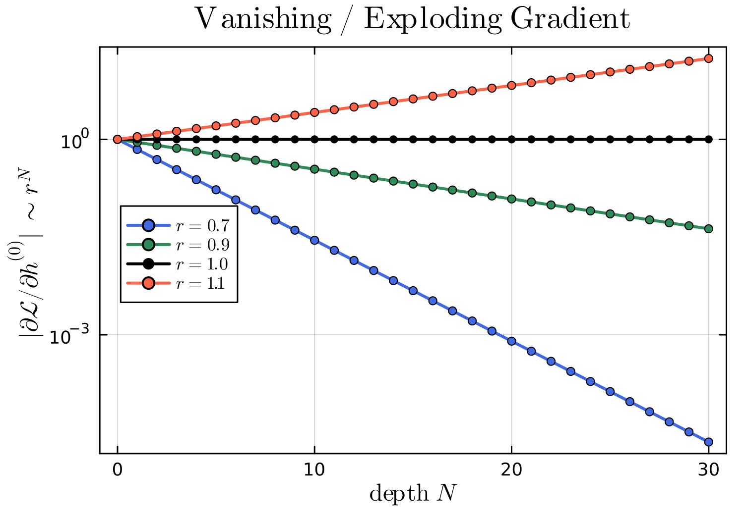
This becomes even clearer with a scalar neural network $h^{(\ell)} = \sigma\left( w^{(\ell)} h^{(\ell-1)} \right)$. In this case the gradient is just a product of real numbers.

$$ \frac{\partial h^{(N)}}{\partial h^{(0)}} = \prod_{k=1}^{N} \sigma^{\prime}\left( z^{(k)} \right) w^{(k)} $$

If the absolute value of each factor is smaller than $1$, the product races exponentially toward $0$; if larger, toward $\infty$.

The Problem with Activation Functions

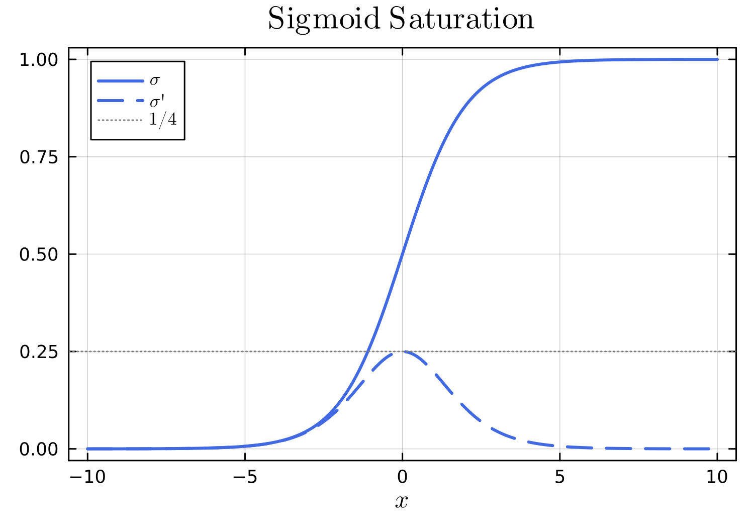
As we saw above, the vanishing gradient occurs when the magnitude of $J^{(k)}$ is too small, and since $D^{(k)} = \operatorname{diag}\left( \sigma^{\prime}(z^{(k)}_{1}), \dots, \sigma^{\prime}(z^{(k)}_{m}) \right)$, we can see that the derivative of the activation function plays an important role. The sigmoid function, widely used in the early days of deep learning, has a gradient close to $0$ when the absolute value of the input is large. Indeed, the derivative of the sigmoid $\sigma$ cannot exceed a maximum of $1/4$, as follows. This behavior, where $|\sigma^{\prime}(x)|$ rapidly approaches $0$ as $|x|$ grows, is called saturation.

$$ \sigma^{\prime}(x) = \sigma(x)\left( 1 - \sigma(x) \right) \le \frac{1}{4} $$

Since the gradient shrinks by at least a factor of $4$ with every layer it passes through, the vanishing gradient inevitably appeared in deep networks. This is one of the main reasons layers could not be stacked deeply in the early days of deep learning.

Mitigation Methods

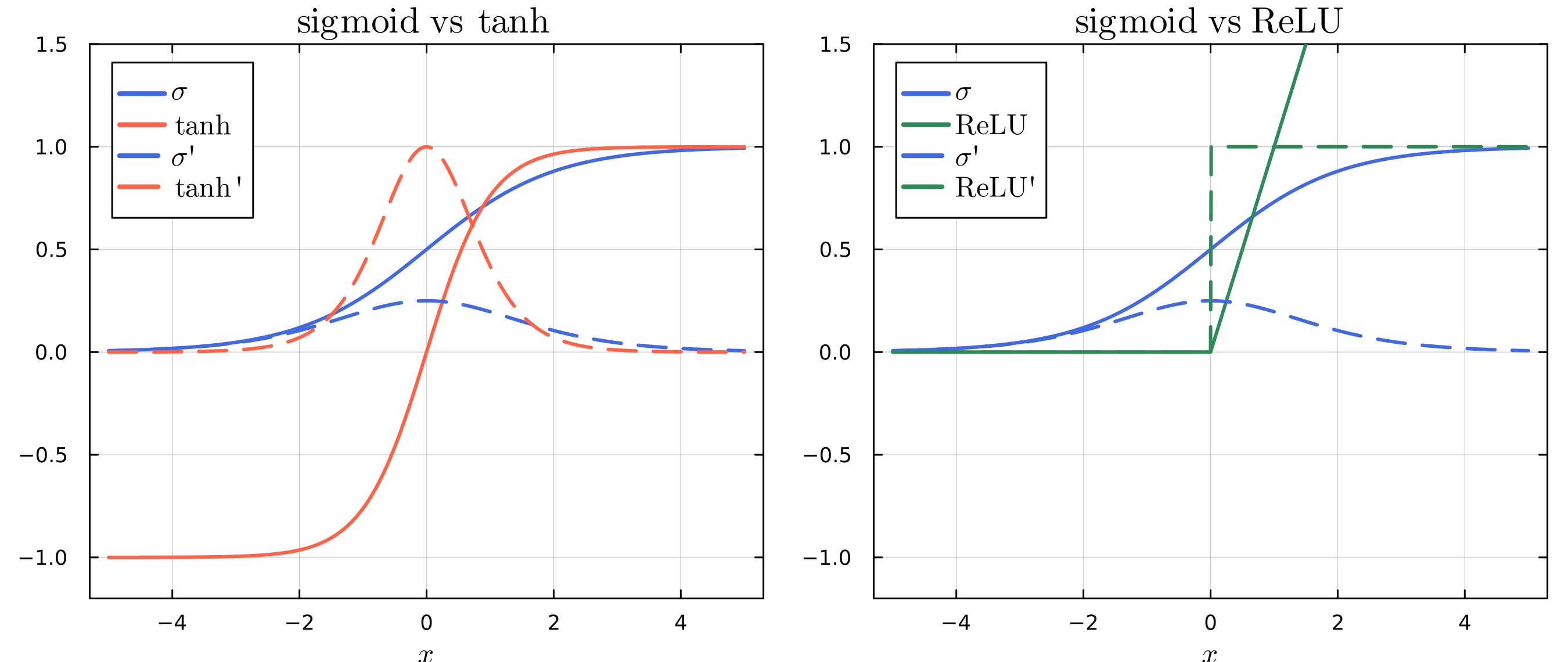
Replacing the activation function: The hyperbolic tangent has a maximum value of $1$ and thus suffers less from the vanishing gradient than the sigmoid, and ReLU has a derivative that is always $1$ in the positive region, greatly alleviating the vanishing gradient.
Skip connection: Adding the identity function to obtain the form $\mathbf{x} \mapsto \sigma(\mathbf{W}\mathbf{x}) + \mathbf{x}$ adds the identity matrix $I$ to the Jacobian matrix, keeping the multiplied terms near $1$. This is the key idea of ResNet, which trained very deep neural networks.
Weight initialization and normalization: Initialization schemes that preserve the variance of values across layers, batch normalization, and the like are used.
Architectural improvements: In recurrent neural networks, the same weight $\mathbf{W}$ is multiplied repeatedly at every time step, so the vanishing gradient is especially severe. LSTM and GRU alleviate this with gate structures that pass the hidden state through addition rather than multiplication.