
Implementing the Discrete Fourier Transform Matrix in Julia
Explanation
The discrete Fourier transform of an $N$-dimensional vector $\mathbf{x}$ is expressed as the following matrix product.
$$ \widehat{\mathbf{x}} = F \mathbf{x} $$
Here $F$, writing $\omega = e^{-i2\pi/N}$, is
$$ F = \begin{bmatrix} 1 & 1 & 1 & \cdots & 1 \\ 1 & \omega & \omega^2 & \cdots & \omega^{N-1} \\ 1 & \omega^2 & \omega^4 & \cdots & \omega^{2(N-1)} \\ \vdots & \vdots & \vdots & \ddots & \vdots \\ 1 & \omega^{N-1} & \omega^{2(N-1)} & \cdots & \omega^{(N-1)^{2}} \end{bmatrix} $$
The inverse transform is expressed as $F^{-1} = \dfrac{1}{N} \overline{F}$. Here $\overline{F}$ is the complex conjugate matrix of $F$.
Implementation
1D Discrete Fourier Transform
In Julia it can be implemented as follows.
function dft_matrix(n)
    ω = exp(-2π*im/n)
    F = [ω^(i*j) for i in 0:n-1, j in 0:n-1]

    return F
end
Of course, it can also be written in a single line as follows.
function dft_matrix(n)
    return [exp(2π *im*i*j/n) for i in 0:n-1, j in 0:n-1]
end
Loading FFTW, the fast Fourier transform package, to check gives the following.
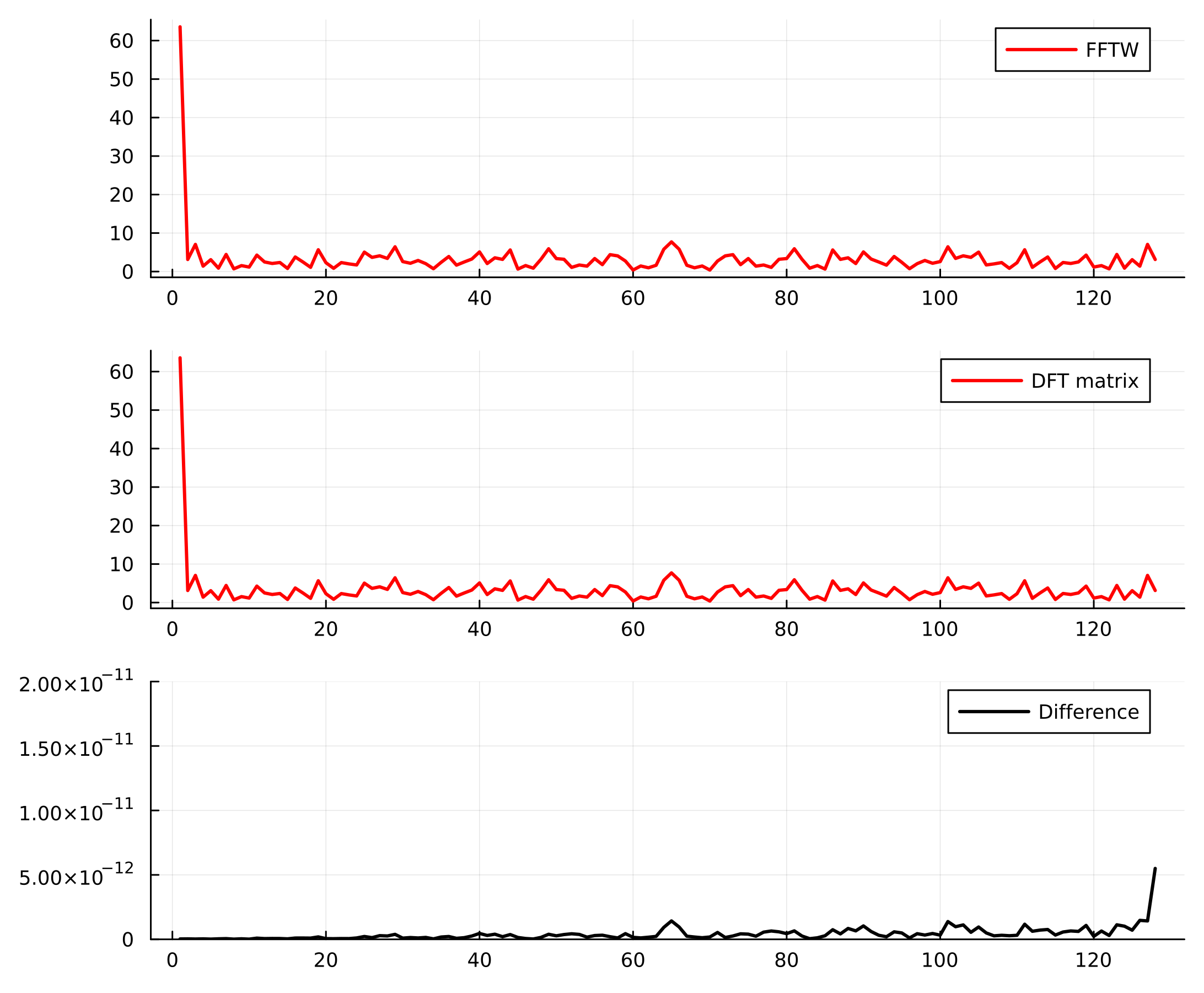
using FFTW
using Plots

F = dft_matrix(128)
x = rand(128)

ξ = fft(x)
η = F*x

plot(
    plot(abs.(ξ), label="FFTW"),
    plot(abs.(η), label="DFT matrix"),
    plot(abs.(ξ .- η), label="Difference"),
    layout=(3,1)
)
2D Discrete Fourier Transform
To implement the two-dimensional transform, let us load an image.
using Tomography

p = phantom(128, 2)
heatmap(p, yflip=true, c=:viridis)
Comparing with FFTW gives the following.
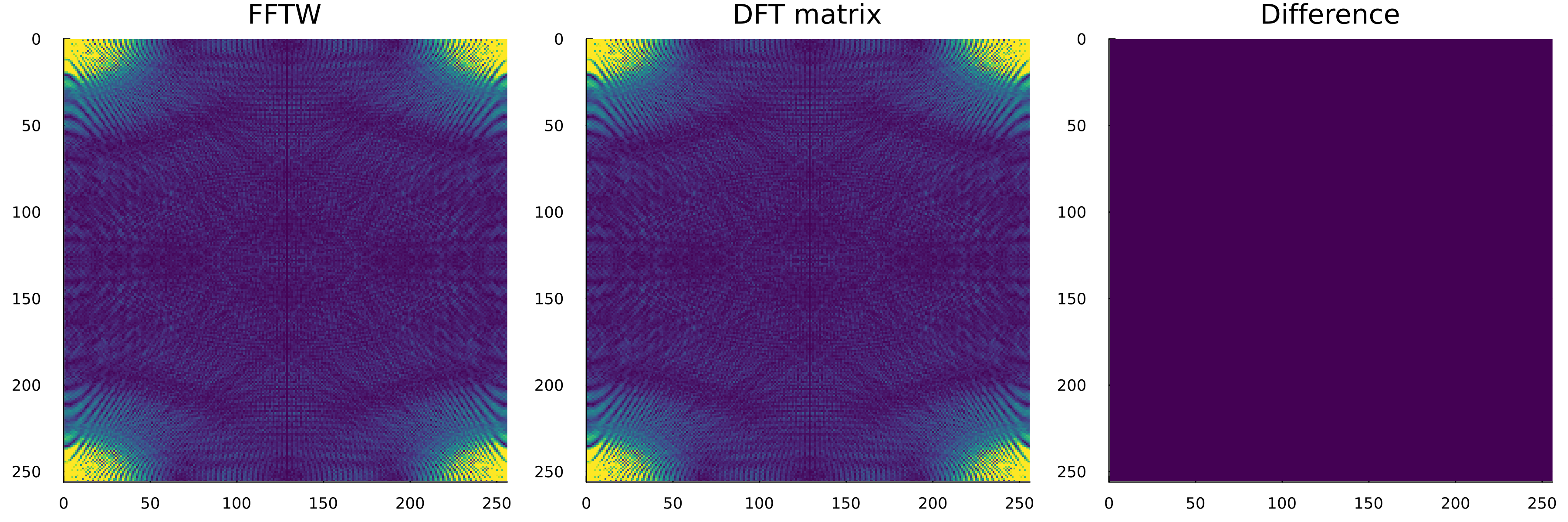
F = dft_matrix(256)
ξ = fft(p)
η = F*p*transpose(F)

plot(
    heatmap(abs.(ξ), yflip=true, title="FFTW"),
    heatmap(abs.(η), yflip=true, aspect_ratio=1, title="DFT matrix"),
    heatmap(abs.(ξ .- η), yflip=true, aspect_ratio=1, title="Difference"),
    layout=(1,3)
)
Inverse Transform
Since the inverse transform is the complex conjugate matrix of the transform matrix, it can be implemented as follows.
function dft_inverse(F)
    n = size(F, 1)
    return conj(F) / n
end

F = dft_matrix(128)
x = rand(128)
F⁻¹ = dft_inverse(F)
plot(
    plot(x, label="Original signal x"),
    plot(real(F⁻¹*F*x), label="Reconstructed signal F⁻¹*F*x"),
    plot(abs.(x .- F⁻¹*F*x), label="Difference"),
    layout = (3,1)
)
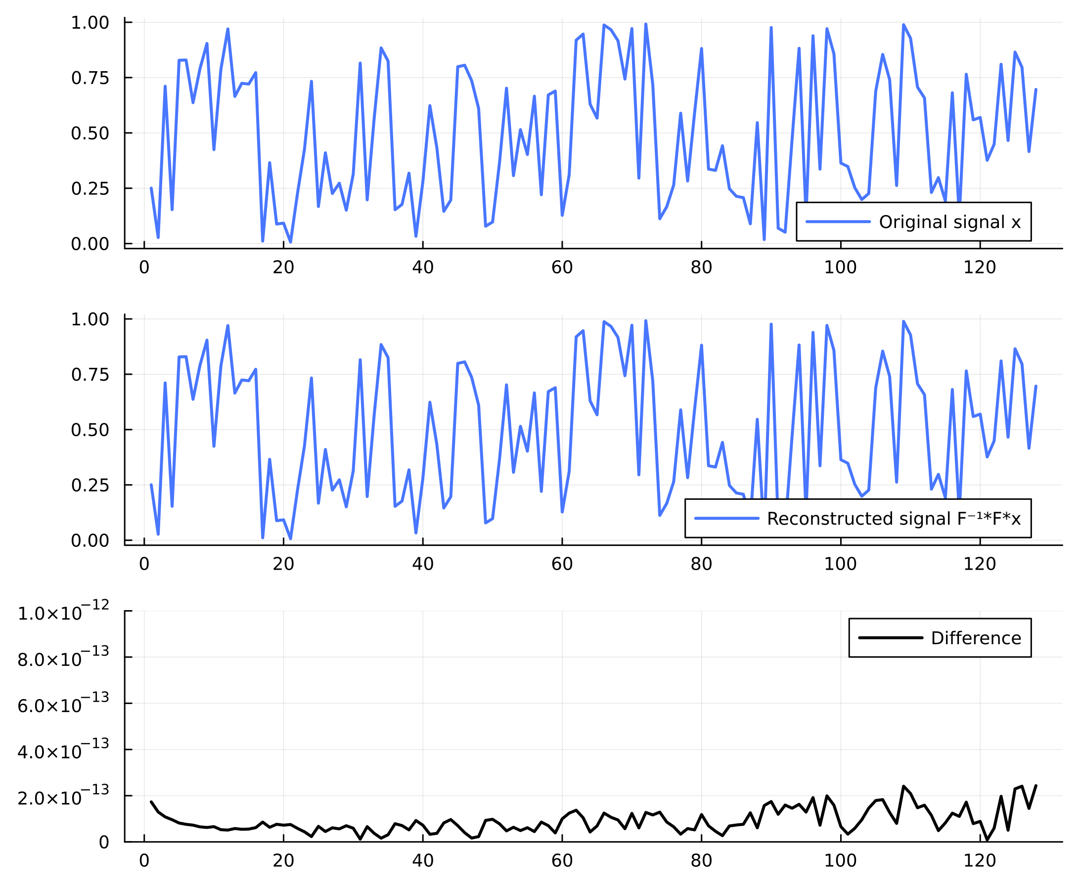
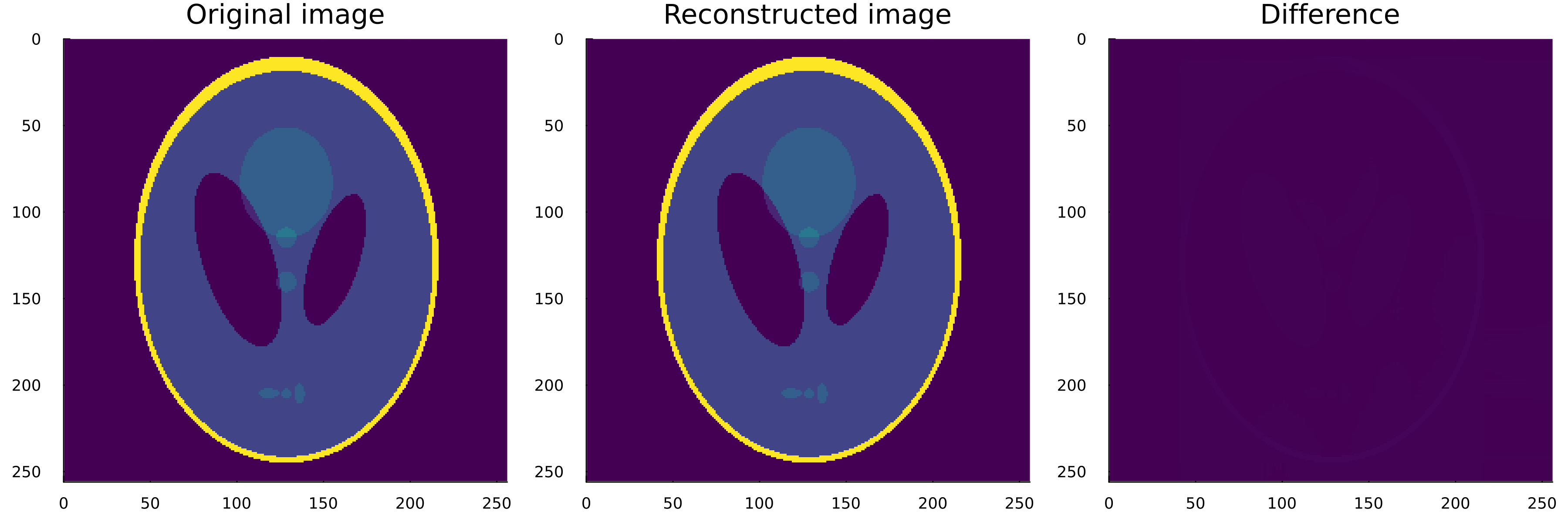
The two-dimensional case is likewise,
p = phantom(256, 2)
F = dft_matrix(256)
F⁻¹ = dft_inverse(F)
p_reconstructed = F⁻¹*F*p*transpose(F)*transpose(F⁻¹)

plot(
    heatmap(p, yflip=true, title="Original image"),
    heatmap(real(p_reconstructed), yflip=true, title="Reconstructed image"),
    heatmap(abs.(p .- real(p_reconstructed)), yflip=true, title="Difference", clims=(0, 1e-10)),
    layout=(1,3)
)
fftshift
The discrete Fourier transform by default puts the component with frequency $0$ first.
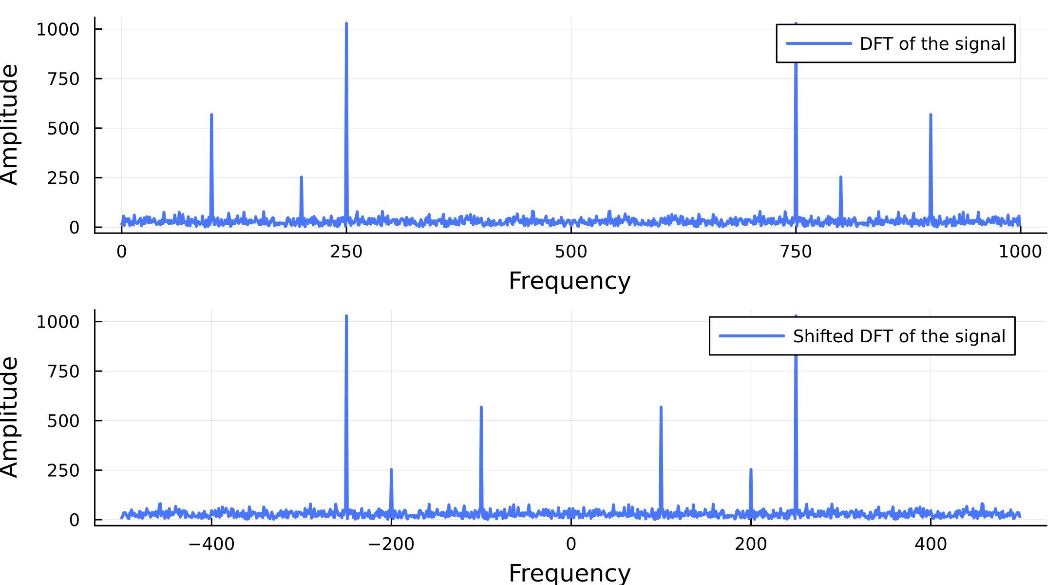
In packages related to the Fourier transform, there is a function that rearranges things so that the $0$ frequency component comes to the center (usually named fftshift); let us implement this.
Since we only need to swap the first half of the components with the second half, it can be implemented easily as follows.
Fs = 1000                    # 진동수
T = 1/1000                   # 샘플링 간격
L = 1000                     # 신호의 길이
x = [i for i in 0:L-1].*T    # 신호의 도메인

F = dft_matrix(L)        # 0 주파수 성분이 첫번째 성분에 오도록 하는 푸리에 변환 행렬
S = shifted_matrix(F)    # 0 주파수 성분이 중앙에 오도록 하는 푸리에 변환 행렬

y₁ = sin.(2π*100*x)            # 진동수가 100인 사인파
y₂ = 0.5sin.(2π*200*x)         # 진동수가 200인 사인파
y₃ = 2sin.(2π*250*x)           # 진동수가 250인 사인파
y = y₁ + y₂ + y₃ + randn(L)    # 잡음이 섞인 신호

ξ = Fs*[i for i in 0:L-1]/L    # 주파수 도메인

plot(
    plot(ξ       , abs.(F*y), label="DFT of the signal"        ),
    plot(ξ .- 500, abs.(S*y), label="Shifted DFT of the signal"),
    layout=(2,1)
)
The result in two dimensions is as follows.
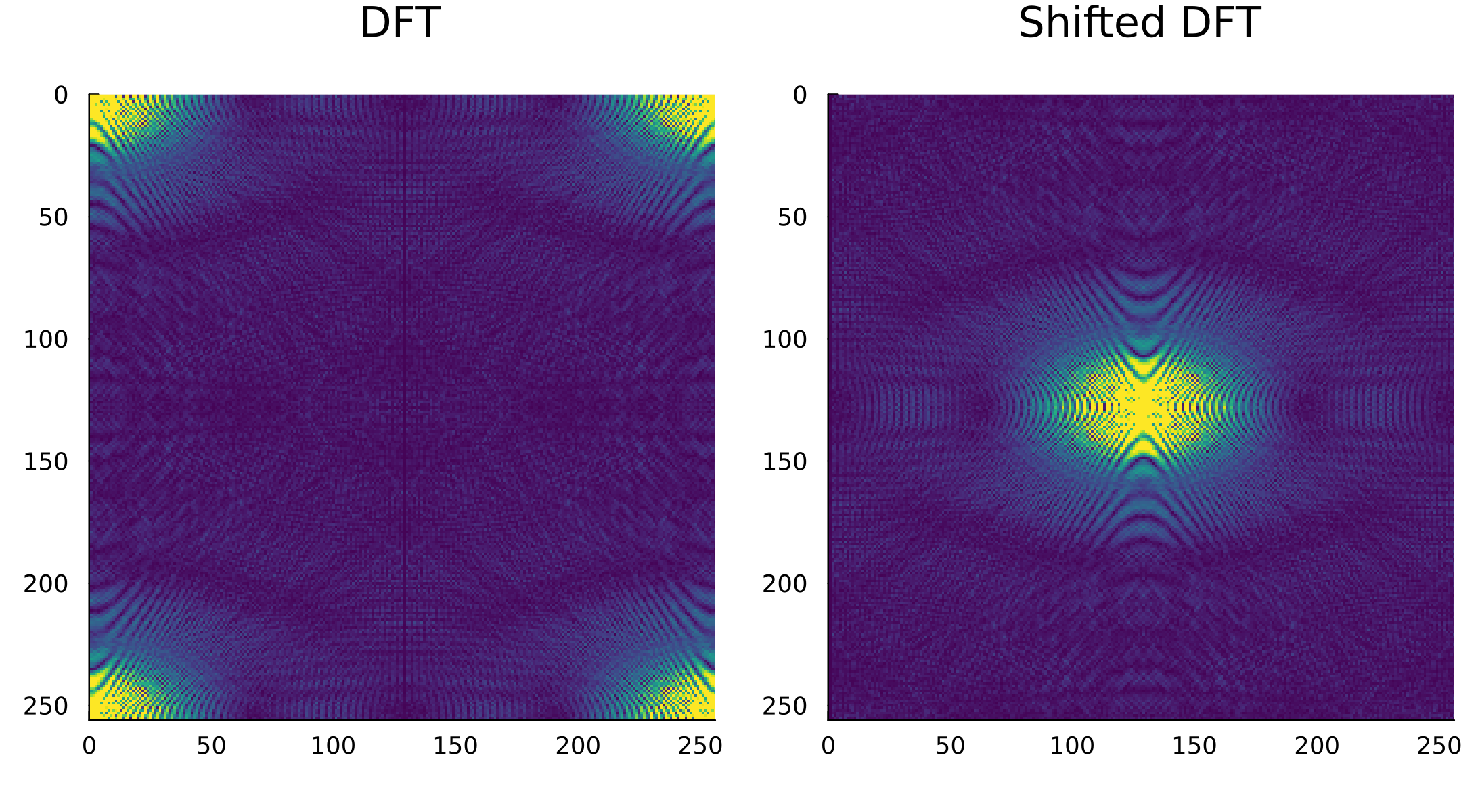
p = phantom(256, 2)
F = dft_matrix(256)
S = shifted_matrix(F)

ξ = F*p*transpose(F)
η = S*p*transpose(S)

plot(
    heatmap(abs.(ξ), yflip=true, clims=(0, 200)),
    heatmap(abs.(η), yflip=true, clims=(0, 200)),
    layout=(1,2),
)
Complete Code
function dft_matrix(n)
    ω = exp(-2π*im/n)
    F = [ω^(i*j) for i in 0:n-1, j in 0:n-1]

    return F
end


function dft_matrix(n)
    return [exp(2π *im*i*j/n) for i in 0:n-1, j in 0:n-1]
end


using FFTW
using Plots

F = dft_matrix(128)
x = rand(128)

ξ = fft(x)
η = F*x

plot(
    plot(abs.(ξ), label="FFTW"),
    plot(abs.(η), label="DFT matrix"),
    plot(abs.(ξ .- η), label="Difference"),
    layout=(3,1)
)


using Tomography

p = phantom(128, 2)
heatmap(p, yflip=true, c=:viridis)


F = dft_matrix(256)
ξ = fft(p)
η = F*p*transpose(F)

plot(
    heatmap(abs.(ξ), yflip=true, title="FFTW"),
    heatmap(abs.(η), yflip=true, aspect_ratio=1, title="DFT matrix"),
    heatmap(abs.(ξ .- η), yflip=true, aspect_ratio=1, title="Difference"),
    layout=(1,3)
)


function dft_inverse(F)
    n = size(F, 1)
    return conj(F) / n
end

F = dft_matrix(128)
x = rand(128)
F⁻¹ = dft_inverse(F)
plot(
    plot(x, label="Original signal x"),
    plot(real(F⁻¹*F*x), label="Reconstructed signal F⁻¹*F*x"),
    plot(abs.(x .- F⁻¹*F*x), label="Difference"),
    layout = (3,1)
)


p = phantom(256, 2)
F = dft_matrix(256)
F⁻¹ = dft_inverse(F)
p_reconstructed = F⁻¹*F*p*transpose(F)*transpose(F⁻¹)

plot(
    heatmap(p, yflip=true, title="Original image"),
    heatmap(real(p_reconstructed), yflip=true, title="Reconstructed image"),
    heatmap(abs.(p .- real(p_reconstructed)), yflip=true, title="Difference", clims=(0, 1e-10)),
    layout=(1,3)
)


Fs = 1000                    # 진동수
T = 1/1000                   # 샘플링 간격
L = 1000                     # 신호의 길이
x = [i for i in 0:L-1].*T    # 신호의 도메인

F = dft_matrix(L)        # 0 주파수 성분이 첫번째 성분에 오도록 하는 푸리에 변환 행렬
S = shifted_matrix(F)    # 0 주파수 성분이 중앙에 오도록 하는 푸리에 변환 행렬

y₁ = sin.(2π*100*x)            # 진동수가 100인 사인파
y₂ = 0.5sin.(2π*200*x)         # 진동수가 200인 사인파
y₃ = 2sin.(2π*250*x)           # 진동수가 250인 사인파
y = y₁ + y₂ + y₃ + randn(L)    # 잡음이 섞인 신호

ξ = Fs*[i for i in 0:L-1]/L    # 주파수 도메인

plot(
    plot(ξ       , abs.(F*y), label="DFT of the signal"        ),
    plot(ξ .- 500, abs.(S*y), label="Shifted DFT of the signal"),
    layout=(2,1)
)


p = phantom(256, 2)
F = dft_matrix(256)
S = shifted_matrix(F)

ξ = F*p*transpose(F)
η = S*p*transpose(S)

plot(
    heatmap(abs.(ξ), yflip=true, clims=(0, 200)),
    heatmap(abs.(η), yflip=true, clims=(0, 200)),
    layout=(1,2),
)
Environment
- OS: Windows11
- Version: Julia 1.10.0, FFTW v1.8.0, Plots v1.40.3, Tomography v0.1.5